Clostridioides difficile is a pathogen found in the gut that can proliferate once antibiotics remove its competing bacteria, leading to recurrent Clostridioides difficile infection (rCDI) Helmholtz Centre for Infection Research. Fecal microbiota transplantation (FMT) treats rCDI by restoring a donor’s balanced gut microbiota in the patient Zanella Terrier et al. 2014. Since bacterial strains within the same species can behave differently, confirming that a bacterium detected in the patient after treatment is the same strain that came from the donor, rather than a different strain of the same species that was already present, requires strain-level resolution rather than species-level identification alone Smillie et al. 2018.
SameStr is a bioinformatic tool that detects shared microbial strains across metagenomic samples by comparing the genetic variation observed at species-specific marker genes. In FMT studies, this allows tracking of strain persistence and engraftment between donor, pre-FMT, and post-FMT samples Podlesny et al. 2022.
rCDI: recurrent Clostridioides difficile infection, caused by C. difficile spores that survive antibiotic treatment and later reactivate.
FMT: fecal microbiota transplantation, a treatment for rCDI that restores a donor’s gut microbiota in the patient.
Strain: a classification within a bacterial species that exhibits distinct genotypic or phenotypic traits.
Clade: a group of organisms in a phylogenetic tree that share a common ancestor and all of its descendants.
SGB (Species-level Genome Bin): a species-level cluster of genomes used by MetaPhlAn 4 to refer to a taxonomic species. SGBs are reported by their bin ID (e.g. t__SGB4285). The t__ prefix indicates it is a species-level clade.
Marker gene: a short genomic sequence specific to a given clade, used by MetaPhlAn to detect that the clade is present in a sample.
SNV profile: the frequency of each nucleotide observed across the aligned reads at every covered position of a clade’s marker genes in a sample, used by SameStr to compare samples.
MVS (Maximum Variant Profile Similarity): Of all positions covered in both samples, the fraction at which the two samples share at least one nucleotide variant.
Persistence: a strain detected in a patient before FMT (pre-FMT) that is still detected in the same patient after treatment (post-FMT).
Engraftment: a strain from the donor that is detected in the patient’s sample after FMT (post-FMT).
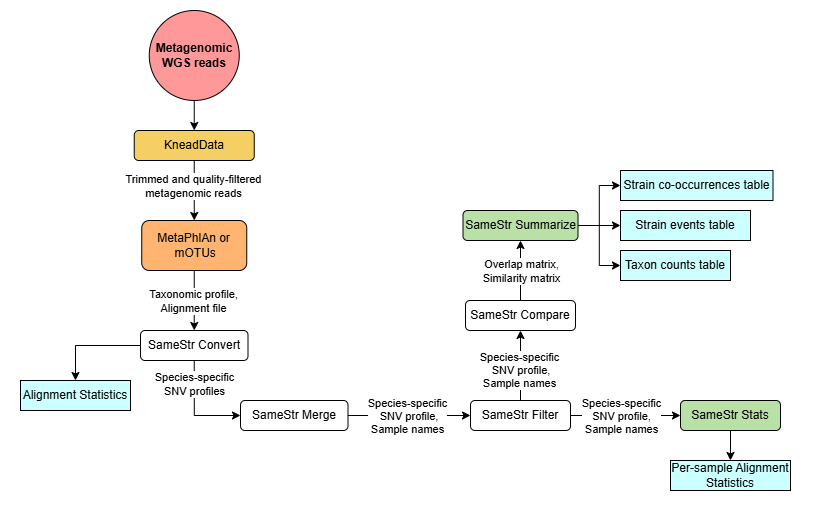
This workflow uses metagenomic samples as input and runs the following sequence of tools to detect shared strains between them:
Reads are trimmed and quality-filtered with KneadData ( Galaxy version 0.12.1+galaxy1).
Reads are aligned to species-specific marker genes with MetaPhlAn ( Galaxy version 4.2.4+galaxy0), which also produces a taxonomic profile for each sample.
The alignments are converted into a species-specific SNV profile for each clade with the SameStr tools.
SNV profiles are merged across samples for each clade.
The Maximum Variant Profile Similarity (MVS) is calculated between samples for each clade.
Overlap and MVS thresholds are applied, and the results are reported in a table across all sample comparisons, indicating whether each clade is classified as a shared strain.
The following sections first go through each tool individually to explain what it does and how it contributes to the entire workflow, and then show how to run the whole thing in one step.
Get data
The following steps use metagenomic shotgun sequencing data from FMT-treated rCDI patient stool samples, part of the FRICKE cohort Podlesny et al. 2022. Three paired-end samples are used: a donor sample, a sample collected from the patient before treatment (pre-FMT), and a sample collected from the patient after treatment (post-FMT). The reads used in this tutorial have been reduced from the original dataset to minimize the time needed to complete the workflow.
Hands On: Data Upload
Create a new history for this tutorial and name it (e.g. “SameStr tutorial”)
To create a new history simply click the new-history icon at the top of the history panel:
Import the files from Zenodo or from
the shared data library (GTN - Material -> microbiome
-> Detection of shared microbial strains with SameStr):
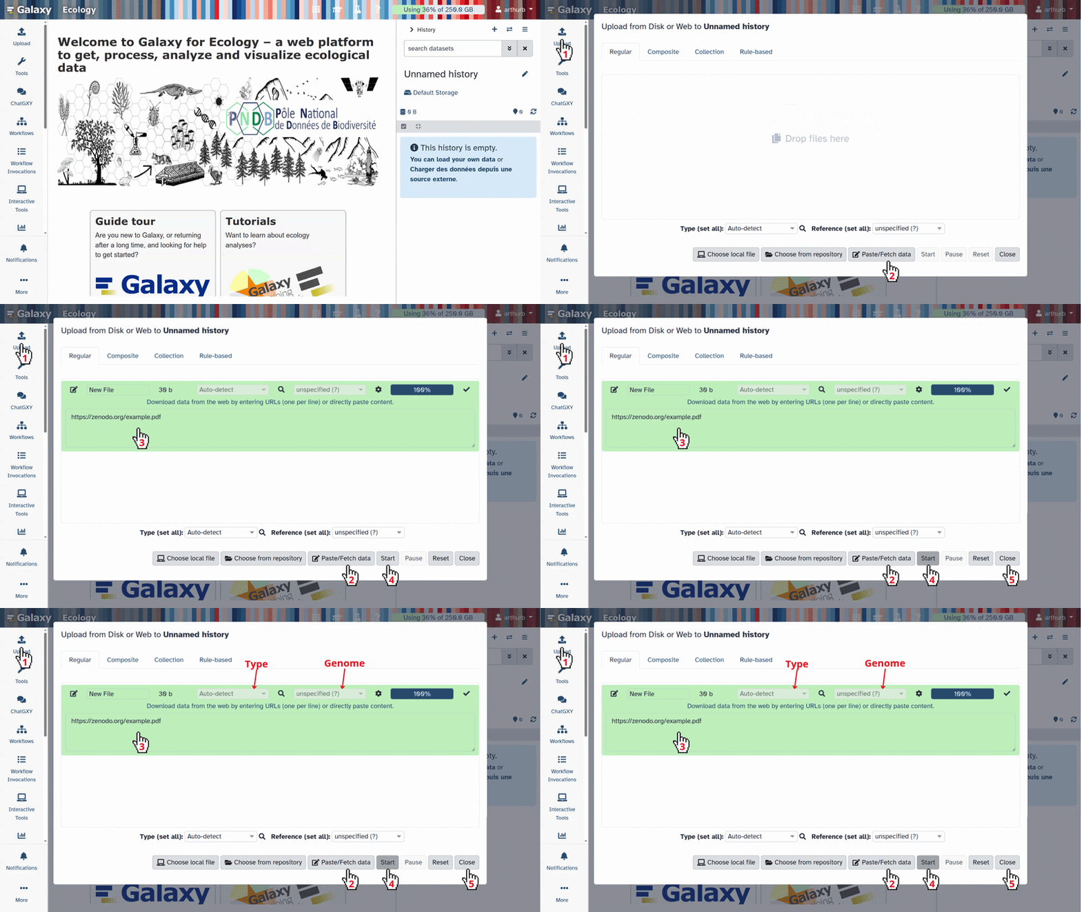
Click galaxy-uploadUpload at the top of the activity panel
Select galaxy-wf-editPaste/Fetch Data
Paste the link(s) into the text field
Press Start
Close the window
As an alternative to uploading the data from a URL or your computer, the files may also have been made available from a shared data library:
Go into Libraries (left panel)
Navigate to the correct folder as indicated by your instructor.
On most Galaxies tutorial data will be provided in a folder named GTN - Material –> Topic Name -> Tutorial Name.
Select the desired files
Click on Add to Historygalaxy-dropdown near the top and select as Datasets from the dropdown menu
In the pop-up window, choose
“Select history”: the history you want to import the data to (or create a new one)
Click on Import
Rename the datasets to show the role of each sample in FMT:
28A_R1 / 28A_R2 → Pre-FMT_R1 / Pre-FMT_R2
28B_R1 / 28B_R2 → Donor_R1 / Donor_R2
28C_R1 / 28C_R2 → Post-FMT_R1 / Post-FMT_R2
Click on the galaxy-pencilpencil icon for the dataset to edit its attributes
In the central panel, change the Name field
Click the Save button
Warning: Non-optional Step
The Apply Rules step later in this tutorial assumes these sample names contain no underscores. Skipping this rename, or keeping the original names, will make Apply Rules silently produce incorrect identifiers.
Check that the datatype of each dataset is set to fastqsanger.gz
Click on the galaxy-pencilpencil icon for the dataset to edit its attributes
In the central panel, click galaxy-chart-select-dataDatatypes tab on the top
In the galaxy-chart-select-dataAssign Datatype, select fastqsanger.gz from “New Type” dropdown
Tip: you can start typing the datatype into the field to filter the dropdown menu
Click the Save button
Build a paired collection from the three samples. Each sample’s forward and reverse reads will be grouped together
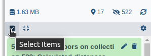
Click on galaxy-selectorSelect Items at the top of the history panel
Check all the datasets in your history you would like to include
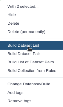
Click n of N selected and choose Advanced Build List
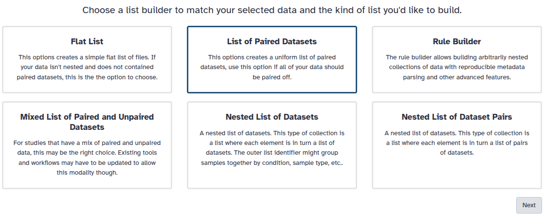
You are in the collection building wizard. Choose List of Paired Datasets and click ‘Next’ button at the right bottom corner.
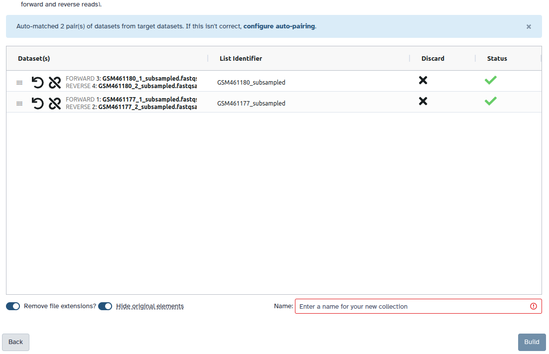
Check and configure auto-pairing. Commonly matepairs have suffix _1 and _2 or _R1 and _R2. Click on ‘Next’ at the bottom.
Edit the List Identifier as required.
Enter a name for your collection
Click Build to build your collection
Click on the checkmark icon at the top of your history again
This section goes through each tool used by SameStr individually, explaining what it does and why it is configured this way. Start with the data uploaded and the paired collection built in the Get data section. Once you’ve been through each tool, you can jump to the end to see how to run the whole thing in one step instead.
Pre-processing of reads with KneadData
KneadData ( Galaxy version 0.12.1+galaxy1) trims reads based on quality parameters and performs host-read removal on the raw sequencing reads The Huttenhower Lab n.d.. This step is performed to reduce the impact of sequencing-quality errors on the shared strain analysis. KneadData has several tools internally, which can be seen as different sections in the tool.
Trimmomatic performs quality-based trimming and removes adapters, short synthetic DNA sequences attached to each read during library preparation so it can bind to the sequencer. These are not part of the original biological sample, so they must be removed before alignment.
Tandem Repeat Finder (TRF) removes repetitive DNA sequences, short sequences repeated consecutively along the genome that can otherwise align to multiple locations and introduce ambiguous mappings.
FastQC reports can be enabled to obtain additional outputs of quality metrics for the sequencing reads.
Host removal discards reads that map to the host genome, since raw metagenomic reads can contain both microbial and human DNA, and only the microbial DNA is relevant for the shared strain analysis.
TRF and FastQC are optional and are skipped in this tutorial, matching how KneadData was configured in the original SameStr publication Podlesny et al. 2022.
Hands On: Trim and Remove Host Reads
KneadData ( Galaxy version 0.12.1+galaxy1) with the following parameters:
“Read type”: Paired reads
“Save all unmatched reads”: Yes
param-collection“Paired reads collection”: the paired collection created earlier
In “Alignment Tool”:
“Select reference genome database”: hg19 (KneadData’s bundled human reference)
“Specify if you want to include the TRF step in the workflow.”: Skip TRF Step
Warning: Understanding KneadData's outputs
KneadData runs quality and adapter trimming (Trimmomatic) and host-DNA removal (Bowtie2) as two sequential steps, and reports the result after each step. Trimmed paired reads and Unmatched trimmed reads are the intermediate result right after trimming only, before host-DNA removal. Paired output reads and Unmatched reads are the final result, after both trimming and host removal. If TRF is enabled, two further output collections are added, containing only the reads affected by repeat removal. These are useful for inspection but are not meant to be carried forward.
Merge collections with the following parameters:
In “Input Collections”:
param-repeat“Insert Input Collections”
param-collection“Input Collection”: Paired output reads (output of KneadDatatool)
param-repeat“Insert Input Collections”
param-collection“Input Collection”: Unmatched reads (output of KneadDatatool)
In “Advanced Options”:
“How should conflicts (or potential conflicts) be handled?”: Keep first instance
Comment: Why merge these two collections?
Of KneadData’s output collections, Paired output reads and Unmatched reads are the final fully decontaminated reads. Merging both ensures that all of the surviving microbial sequence data is used in the strain-level analysis, since orphaned reads also carry valuable information.
Question
Why is hg19, a human reference genome, selected as the reference genome database for host removal?
Because the samples used are human stool, so the sequencing reads include human DNA alongside the microbial DNA. This human DNA must be removed before the strain analysis.
The result of these two steps is a single collection containing one set of reads per sample: all the reads that passed KneadData’s quality filtering and host decontamination, both paired and orphaned. The reads are now ready to be used for taxonomic profiling in the next step.
Taxonomic profiling and marker-based alignment with MetaPhlAn
MetaPhlAn ( Galaxy version 4.2.4+galaxy0) performs both the taxonomic profiling and the marker-based alignment used by SameStr. It maps the pre-processed reads against a set of clade-specific markers derived from reference genomes Blanco-Míguez et al. 2023. MetaPhlAn produces several outputs. The ones used in the subsequent workflow steps are the taxonomic profile, which lists the relative abundance of each clade detected in the sample, and the reads that aligned to the markers.
Hands On: Taxonomic profiling and Read Alignment
MetaPhlAn ( Galaxy version 4.2.4+galaxy0) with the following parameters:
In “Inputs”:
“Input(s)”: Fasta/FastQ file(s) with microbiota reads
“Fasta/FastQ file(s) with microbiota reads”: Paired-end collection
param-collection“Paired-end Fasta/FastQ file with microbiota reads”: the paired collection produced by Merge collectionstool
“Database with clade-specific marker genes”: Locally cached
“Cached database with clade-specific marker genes”: mpa_vJan25_CHOCOPhlAnSGB_202503-11062025
Samtools view ( Galaxy version 1.22+galaxy2) with the following parameters:
param-collection“SAM/BAM/CRAM data set”: SAM file collection (output of MetaPhlAntool)
“What would you like to look at?”: All reads in the input dataset
“What would you like to have reported?”: The actual reads
“Output format”: BAM (-b)
“Use a reference sequence”: No
Click on param-collectionDataset collection in front of the input parameter you want to supply the collection to.
Select the collection you want to use from the list
Comment: Why convert to BAM?
MetaPhlAn outputs the aligned reads in SAM format, but SameStr Convert requires BAM input. Samtools performs this conversion.
The taxonomic profile identifies which clades are present in each sample and at what relative abundance. SameStr can only compare strains for a clade if that clade is detected in more than one sample, so the taxonomic profile determines, for each pair of samples, which clades are even candidates for shared strain detection in the following steps.
Strain-level analysis with SameStr
SameStr is not a single tool but a chain of command-line tools, each carrying out one step of the shared-strain detection process. The chain starts with the marker alignments, which are converted into per-clade SNV profiles. These profiles are then merged across samples and filtered to remove low-quality positions, before the samples are compared to identify shared strains between them. The following subsections go through each of these tools in the order they are run.
SameStr Convert
SameStr Convert ( Galaxy version 1.2025.111+galaxy0) takes the aligned reads and the taxonomic profile from MetaPhlAn and produces one SNV profile per detected clade, describing the nucleotides observed at each covered position of that clade’s marker genes.
Hands On: Generate Per-Clade SNV Profiles
SameStr Convert ( Galaxy version 1.2025.111+galaxy0) with the following parameters:
param-collection“Aligned reads”: filtered alignments collection produced by Samtools viewtool
param-collection“Taxonomic profile”: Predicted taxon relative abundances collection produced by MetaPhlAntool
Comment: What do these alignment parameters control?
Each of these settings decides whether a given aligned read, or a given position within it, has enough quality to be counted in the SNV profile:
“Percent identity” is the minimum fraction of bases in a read that must match the reference marker sequence. Reads with more mismatches than this are discarded.
“Minimum alignment length” is the shortest amount of aligned base pairs a read can have and still be kept. Shorter alignments are considered too unreliable to use.
“Minimum base quality” is the lowest sequencing quality score a nucleotide call can have and still be counted. A score of 20 corresponds to a 99% probability that the base was called correctly.
“Minimum alignment quality” is the lowest mapping quality score a read can have and still be kept. Setting it to 0 means no read is excluded on this basis alone.
“Minimum vertical coverage” is the minimum number of reads that must cover a position for that position to be included in the SNV profile.
Sequencing quality scores follow the Phred scale, where the score Q relates to the probability P of an incorrect base call by Q = -10·log₁₀(P). For a quality score of 20, this gives P = 10⁻² = 0.01, a 1% chance of an incorrect call.
Each run of SameStr Convert produces two outputs. The per-clade SNV profiles are compressed NumPy arrays (.npz) that have the nucleotide frequencies observed at every covered position of one clade’s marker genes in this sample. The second output generated is the alignment statistics table. For each clade it reports the mean and median coverage, the number of covered positions, and the fraction of those positions that are monomorphic versus polymorphic (f_mono/f_poly).
Question
Open the alignment statistics table for one of your samples. Are the clades mostly monomorphic or polymorphic?
Mostly monomorphic: f_mono is close to 1.0 and f_poly close to 0.0 for most clades, meaning each clade is dominated by a single strain in this sample.
Hands On: Flatten the SNV Profile Collection
Flatten collection with the following parameters:
param-collection“Input Collection”: per-clade SNV profiles collection produced by SameStr Converttool
SameStr Convert organizes its output by sample, with each sample containing one npz file per detected clade. SameStr Merge instead needs a single flat list of npz files, since it groups them by clade internally based on their filenames. Flatten collection removes the per-sample nesting so all npz files can be passed to SameStr Merge together.
The Flatten collection tool joins each identifier with an underscore, which adds the sample name as an extra prefix, producing sample_clade.sample (e.g. Pre-FMT_t__SGB14809.Pre-FMT). This breaks the clade.sample format that SameStr Merge expects, so the following step removes this prefix and restores the original identifiers. The step is added to the workflow as a workaround for Apply Rules’ flat-list input requirement.
Hands On: Fix the Collection Identifiers
Apply rules with the following parameters:
param-collection“Input Collection”: the flattened SNV profile collection produced by Flatten collectiontool
Under “Rules” click “galaxy-wf-edit Edit” to open the Rule Builder
Click “plus Column” -> “Using a Regular Expression”
In “From Column”, choose A from the dropdown
Select “Create column from expression replacement”
Fill in “Regular Expression”: ^[^_]+_(.*)$
Fill in “Replacement Expression”: \1
Regular expressions are a standardized way of describing patterns in textual data. They can be extremely useful for tasks such as finding and replacing data. They can be a bit tricky to master, but learning even just a few of the basics can help you get the most out of Galaxy.
Finding
Below are just a few examples of basic expressions:
Regular expression
Matches
abc
an occurrence of abc within your data
(abc|def)
abcordef
[abc]
a single character which is either a, b, or c
[^abc]
a character that is NOT a, b, nor c
[a-z]
any lowercase letter
[a-zA-Z]
any letter (upper or lower case)
[0-9]
numbers 0-9
\d
any digit (same as [0-9])
\D
any non-digit character
\w
any alphanumeric character
\W
any non-alphanumeric character
\s
any whitespace
\S
any non-whitespace character
.
any character
\.
literal . (period)
{x,y}
between x and y repetitions
^
the beginning of the line
$
the end of the line
Note: you see that characters such as *, ?, ., + etc have a special meaning in a regular expression. If you want to match on those characters, you can escape them with a backslash. So \? matches the question mark character exactly.
Examples
Regular expression
matches
\d{4}
4 digits (e.g. a year)
chr\d{1,2}
chr followed by 1 or 2 digits
.*abc$
anything with abc at the end of the line
^$
empty line
^>.*
Line starting with > (e.g. Fasta header)
^[^>].*
Line not starting with > (e.g. Fasta sequence)
Replacing
Sometimes you need to capture the exact value you matched on, in order to use it in your replacement, we do this using capture groups (...), which we can refer to using \1, \2 etc for the first and second captured values. If you want to refer to the whole match, use &.
Regular expression
Input
Captures
chr(\d{1,2})
chr14
\1 = 14
(\d{2}) July (\d{4})
24 July 1984
\1 = 24, \2 = 1984
An expression like s/find/replacement/g indicates a replacement expression, this will search (s) for any occurrence of find, and replace it with replacement. It will do this globally (g) which means it doesn’t stop after the first match.
Example: s/chr(\d{1,2})/CHR\1/g will replace chr14 with CHR14 etc.
You can also use replacement modifier such as convert to lower case \L or upper case \U. Example: s/.*/\U&/g will convert the whole text to upper case.
Note: In Galaxy, you are often asked to provide the find and replacement expressions separately, so you don’t have to use the s/../../g structure.
There is a lot more you can do with regular expressions, and there are a few different flavours in different tools/programming languages, but these are the most important basics that will already allow you to do many of the tasks you might need in your analysis.
Tip:RegexOne is a nice interactive tutorial to learn the basics of regular expressions.
Tip:Regex101.com is a great resource for interactively testing and constructing your regular expressions, it even provides an explanation of a regular expression if you provide one.
Tip:Cyrilex is a visual regular expression tester.
Warning: Sample Names Must Not Contain Underscores
The regex ^[^_]+_(.*)$ strips everything up to the first underscore, treating it as the sample-name prefix added by Flatten collection. This only works if sample names themselves contain no underscores. If your own sample names contain underscores, this step will strip too much, please avoid underscores in your naming, or adjust the regex accordingly.
Comment: Expected output
If you are following this tutorial with the same parameters and datasets, you should have a single flat list of 28 npz datasets, combining all samples together.
SameStr Merge
SameStr Merge ( Galaxy version 1.2025.111+galaxy0) combines the per-sample SNV profiles for the same clade into a single multi-sample profile. For each clade, it produces one merged npz profile combining the data from every sample that contains it, along with a sample name file listing which samples are included.
Hands On: Merge SNV Profiles Across Samples
SameStr Merge ( Galaxy version 1.2025.111+galaxy0) with the following parameters:
param-collection“Input SNV profiles”: the SNV profile collection produced by Apply rulestool
Click on param-collectionDataset collection in front of the input parameter you want to supply the collection to.
Select the collection you want to use from the list
Question
The input to SameStr Merge was a list of 28 npz datasets. After running SameStr Merge, this list decreased to 22 datasets. Why do we have fewer datasets than before?
SameStr Merge combines the per-sample profiles for the same clade into a single profile, so any clade detected in more than one sample is merged into one entry instead of being counted once per sample.
SameStr Filter
SameStr Filter ( Galaxy version 1.2025.111+galaxy0) removes clades, samples, and positions that do not meet a set of coverage and quality thresholds, before the profiles are used to detect shared strains.
Hands On: Filter the Merged SNV Profiles
SameStr Filter ( Galaxy version 1.2025.111+galaxy0) with the following parameters:
param-collection“SNV profile to filter”: per-clade merged SNV profiles collection produced by SameStr Mergetool
param-collection“Sample identifiers”: per-clade sample names collection produced by SameStr Mergetool
“Position coverage standard deviation cutoff”: 3.0
In “Sample Filtering”:
“Minimum horizontal coverage (nucleotides)”: 5000
In “Global Position Filtering”:
“Minimum sample coverage per position (count)”: 2
Comment: What do these filtering parameters control?
“Minimum samples per clade” discards clades detected in fewer samples than this.
“Marker truncation length” trims this many nucleotides from each end of every marker gene, removing edge regions where alignments tend to be less reliable.
“Minimum variant coverage” (nucleotides and fraction) sets the minimum read count and minimum proportion of reads that must support a nucleotide call for it to be counted as a real variant, rather than sequencing noise.
“Minimum position coverage” and the “standard deviation cutoff” remove positions with too few reads, or with coverage that is too high or too low than a sample’s average.
“Minimum horizontal coverage” discards a clade from a sample if too few of its marker positions are covered overall.
“Minimum sample coverage per position” keeps a position in the final profile only if it is covered in at least this many samples.
The resulting collections contain some empty datasets. In order to use the collections in the subsequent steps, the empty datasets need to be eliminated from the collections.
Hands On: Remove Empty Datasets
Filter empty datasets with the following parameters:
param-collection“Input Collection”: filtered SNV profiles produced by SameStr Filtertool
Filter empty datasets with the following parameters:
param-collection“Input Collection”: per-clade retained sample names produced by SameStr Filtertool
Comment: Expected output
If you are following this tutorial with the same parameters and datasets, you should now have 3 datasets in the filtered SNV profile collection, and 3 tabular datasets in the sample name collection.
SameStr Stats
SameStr Stats ( Galaxy version 1.2025.111+galaxy0) is a side branch of the workflow: its output is a final result and is not consumed by any later tool. It calculates statistics on the coverage and nucleotide diversity of the filtered SNV profiles.
Hands On: Compute Alignment Statistics
SameStr Stats ( Galaxy version 1.2025.111+galaxy0) with the following parameters:
param-collection“Input SNV profiles”: the SNV profile collection produced by Filter empty datasetstool
param-collection“Sample identifiers”: the sample name collection produced by Filter empty datasetstool
Two columns are especially useful for a first look at the results. f_covered shows what fraction of the clade’s marker positions were actually covered in a given sample, which reflects how much of that clade was captured by sequencing. f_mono and f_poly show whether the covered positions are dominated by a single nucleotide (monomorphic) or contain multiple nucleotides (polymorphic). A high f_mono value suggests the sample is colonized by a single dominant strain for that clade, while a higher f_poly value would point to multiple co-existing strains.
Question
Looking at your SameStr Stats output, for each clade, are the covered positions monomorphic or polymorphic? How can you tell?
Monomorphic. For every clade and every sample, f_mono is 1.0 and f_poly is 0.0, meaning all covered positions are dominated by a single nucleotide, with no positions showing multiple co-occurring variants.
SameStr Compare
SameStr Compare ( Galaxy version 1.2025.111+galaxy0) calculates pairwise similarity between samples for each clade, using the filtered SNV profiles to determine whether samples share the same strain. SameStr Compare generates 3 output matrices for each clade: an overlap matrix giving the number of shared covered positions between each pair of samples, a fraction matrix giving the Maximum Variant Profile Similarity (MVS) between each pair, and a closest matrix identifying each sample’s most similar match.
Hands On: Compare Samples for Each Clade
SameStr Compare ( Galaxy version 1.2025.111+galaxy0) with the following parameters:
param-collection“Input SNV profiles”: the SNV profile collection produced by Filter empty datasetstool
param-collection“Sample identifiers”: the sample name collection produced by Filter empty datasetstool
This step is run with the default setting, which uses all variants without distinguishing between minority and dominant alleles. Two other options exist: using only dominant variants at each position, or using all variants while also reporting a separate set of metrics based on dominant variants alone. A further option, disabled by default, additionally generates FASTA alignments of the dominant variants for each clade as an extra output.
SameStr Summarize
SameStr Summarize ( Galaxy version 1.2025.111+galaxy0) is the last tool in the workflow, which produces the shared-strain results. It combines the overlap and similarity matrices from SameStr Compare with the taxonomic profiles from MetaPhlAn, and generates three summary tables: a taxon count table listing the clades detected per sample, a co-occurrence table showing which clades are shared between sample pairs, and a strain events table reporting, for each shared clade, whether the two samples count as sharing the same strain.
Hands On: Generate the Shared Strain Summary
SameStr Summarize ( Galaxy version 1.2025.111+galaxy0) with the following parameters:
param-collection“Overlap metrics (collection output of SameStr compare)”: Coverage overlap collection produced by SameStr Comparetool
param-collection“Fractional similarities (collection output of SameStr compare)”: Similarity fraction collection produced by SameStr Comparetool
param-collection“Taxonomic profiles”: Predicted taxon relative abundances collection produced by MetaPhlAntool
In “Summary threshold arguments”:
“Minimum overlap for comparison”: 5000
“Minimum similarity for shared strains”: 0.999
Comment: What do these two thresholds control?
These are the two values that decide whether a clade counts as a shared strain between two samples or not.
“Minimum overlap for comparison” (5000) requires at least this many shared covered positions between two samples before their similarity is even considered, so the comparison isn’t based on too little data to be reliable.
“Minimum similarity for shared strains” (0.999) is the MVS threshold a sample pair must have to be classified as sharing a strain.
Interpreting the results from SameStr Summarize
Taxon counts table
This table shows how many different taxa were detected in each sample at every taxonomic level, from kingdom down to clade. It gives a quick way to compare the overall taxonomic groups found in each sample before looking at any shared-strain results. Open the Taxon counts dataset in your own history to see your results. The image below shows an example.
Figure 3: Number of taxa detected in each sample at each taxonomic level.
Co-occurrence table
This table is the fastest way to check whether clades are shared at all between samples. shared_species and shared_clade count how many taxa were detected in both samples, regardless of whether they turned out to be the same strain, while shared_strain counts only those clades confirmed as the same strain by SameStr Compare. The gap between shared_clade and shared_strain tells you how many shared taxa were only confirmed at the species/clade level instead of being detected as strains. Open the Strain co-occurrences dataset in your own history to see your results. The image below shows an example.
Figure 4: Shared taxa between each pair of samples, from kingdom down to strain level.
Question
Why is it less likely that Pre-FMT and Donor share the same strain, compared to the other two pairs?
Can you tell from this table whether any strain persisted in the patient? How would you tell?
The Pre-FMT sample reflects the patient’s gut microbiome before treatment, while the Donor reflects a healthy and unrelated microbiome. These two have no direct biological relationship, so any shared strain between them would be coincidental.
Yes. The Pre-FMT/Post-FMT row shows shared_strain = 0, so no clade was confirmed as the same strain between those samples, this data shows no evidence of persistence.
Strain events table
This table shows the exact clades analyzed between each pair of samples, which is what the co-occurrence table’s totals are built from. Each clade is given one of three events:
shared_strain: when both the overlap and similarity thresholds are met
other_strain: when the overlap threshold is met but similarity falls below 0.999
same_clade: when the overlap threshold itself is not met, so the comparison never reaches strain-level resolution
Open the Strain events dataset in your own history to see your results and compare them to the image below.
Figure 5: Per-clade pairwise comparisons showing overlap, similarity, and the resulting shared-strain classification.
Question
In your results, find a clade with a similarity of 1.0, a perfect match, that is still not labeled shared_strain. Why not?
Its overlap is below the minimum overlap threshold of 5000, so the comparison could only be resolved at clade level, not strain level. That means we can confirm the same clade was found in both samples, but not whether it’s the same strain.
Open your Strain events results and find the one clade classified as shared_strain. This is the shared strain between the Donor and Post-FMT samples, meaning it successfully engrafted.
Running SameStr as a complete workflow
Now that you have run through each step individually, this section shows how to repeat the same analysis in a single step using the published workflow.
Hands On: Run SameStr
Run the SameStrworkflow workflow using the parameter values described in the previous section, tool by tool
param-collection“Raw Reads”: the paired collection built in the Get data step
Click on galaxy-workflows-activityWorkflows in the Galaxy activity bar (on the left side of the screen, or in the top menu bar of older Galaxy instances). You will see a list of all your workflows
Click on galaxy-uploadImport at the top-right of the screen
Paste the following URL into the box labelled “Archived Workflow URL”: https://training.galaxyproject.org/training-material/topics/microbiome/tutorials/samestr-strain-detection/workflows/samestr-strain-detection.ga
Click the Import workflow button
Below is a short video demonstrating how to import a workflow from GitHub using this procedure:
Video: Importing a workflow from URL
These values include some of the parameters mentioned in the original SameStr publication Podlesny et al. 2022. For parameters not specified there, the tool’s default values are used instead. A few important parameters are:
“Select SameStr database” must always match the profiler selected in “Select MetaPhlAn Database”. Mixing databases from different profilers will cause errors.
“Minimum overlap for comparison” (5000) and “Minimum similarity for shared strains” (0.999) are the two thresholds that ultimately decide whether a clade is classified as a shared strain.
The remaining alignment and filtering parameters are explained individually, tool by tool, in the previous section.
Warning: Changing Parameters
The tutorial dataset was reduced to the minimum size that still produces results with the parameter values listed above. Changing these parameters may therefore cause the workflow to produce no output. To experiment with different parameter values, download the complete samples from the ENA under accession PRJEB39023 and repeat the Data Upload step with the full dataset.
Conclusion
This tutorial showed how to detect shared microbial strains between metagenomic samples using SameStr, both as a complete workflow and as individual tools:
Trimming and host-read removal with KneadData ( Galaxy version 0.12.1+galaxy1)
Taxonomic profiling and marker-based alignment with MetaPhlAn ( Galaxy version 4.2.4+galaxy0)
Strain-level SNV profiling, filtering, and comparison with the SameStr tools
Applying this to the FMT-treated rCDI dataset used here, SameStr found one shared strain between the Donor and Post-FMT samples, indicating that this strain successfully engrafted.
You've Finished the Tutorial
Please also consider filling out the Feedback Form as well!
Key points
SameStr enables shared strain detection between metagenomic samples
SameStr can be run as a complete workflow or tool by tool to understand each analysis step
Shared strains are identified by comparing the genetic variation of species-specific marker genes between samples
In FMT-treated rCDI samples, shared strains between donor and post-FMT samples indicate engraftment, while shared strains between pre-FMT and post-FMT samples indicate persistence
Frequently Asked Questions
Have questions about this tutorial? Have a look at the available FAQ pages and support channels
Further information, including links to documentation and original publications, regarding the tools, analysis techniques and the interpretation of results described in this tutorial can be found here.
References
Zanella Terrier, M. C., M. L. Simonet, P. Bichard, and J. L. Frossard, 2014 Recurrent Clostridium difficile infections: The importance of the intestinal microbiota. World Journal of Gastroenterology 20: 7416–7423. 10.3748/wjg.v20.i23.7416
Smillie, C. S., J. Sauk, D. Gevers, J. Friedman, J. Sung et al., 2018 Strain tracking reveals the determinants of bacterial engraftment in the human gut following fecal microbiota transplantation. Cell Host & Microbe 23: 229–240.e5. 10.1016/j.chom.2018.01.003
Podlesny, D., C. Arze, E. Dörner, S. Verma, S. Dutta et al., 2022 Metagenomic strain detection with SameStr: Identification of a persisting core gut microbiota transferable by fecal transplantation. Microbiome 10: 53. 10.1186/s40168-022-01251-w
Blanco-Míguez, A., F. Beghini, F. Cumbo, L. J. McIver, K. N. Thompson et al., 2023 Extending and improving metagenomic taxonomic profiling with uncharacterized species using MetaPhlAn 4. Nature Biotechnology 41: 1633–1644. 10.1038/s41587-023-01688-w
Did you use this material as an instructor? Feel free to give us feedback on how it went.
Did you use this material as a learner or student? Click the form below to leave feedback.
Hiltemann, Saskia, Rasche, Helena et al., 2023 Galaxy Training: A Powerful Framework for Teaching! PLOS Computational Biology 10.1371/journal.pcbi.1010752
Batut et al., 2018 Community-Driven Data Analysis Training for Biology Cell Systems 10.1016/j.cels.2018.05.012
@misc{microbiome-samestr-strain-detection,
author = "Xenia Morera Martínez",
	title = "Detection of shared microbial strains with SameStr (Galaxy Training Materials)",
	year = "",
	month = "",
	day = "",
	url = "\url{https://training.galaxyproject.org/training-material/topics/microbiome/tutorials/samestr-strain-detection/tutorial.html}",
	note = "[Online; accessed TODAY]"
}
@article{Hiltemann_2023,
	doi = {10.1371/journal.pcbi.1010752},
	url = {https://doi.org/10.1371%2Fjournal.pcbi.1010752},
	year = 2023,
	month = {jan},
	publisher = {Public Library of Science ({PLoS})},
	volume = {19},
	number = {1},
	pages = {e1010752},
	author = {Saskia Hiltemann and Helena Rasche and Simon Gladman and Hans-Rudolf Hotz and Delphine Larivi{\`{e}}re and Daniel Blankenberg and Pratik D. Jagtap and Thomas Wollmann and Anthony Bretaudeau and Nadia Gou{\'{e}} and Timothy J. Griffin and Coline Royaux and Yvan Le Bras and Subina Mehta and Anna Syme and Frederik Coppens and Bert Droesbeke and Nicola Soranzo and Wendi Bacon and Fotis Psomopoulos and Crist{\'{o}}bal Gallardo-Alba and John Davis and Melanie Christine Föll and Matthias Fahrner and Maria A. Doyle and Beatriz Serrano-Solano and Anne Claire Fouilloux and Peter van Heusden and Wolfgang Maier and Dave Clements and Florian Heyl and Björn Grüning and B{\'{e}}r{\'{e}}nice Batut and},
	editor = {Francis Ouellette},
	title = {Galaxy Training: A powerful framework for teaching!},
	journal = {PLoS Comput Biol}
}
Congratulations on successfully completing this tutorial!
You can use Ephemeris's shed-tools install command to install the tools used in this tutorial.

 Xenia Morera Martínez

Questions:
 Open image in new tab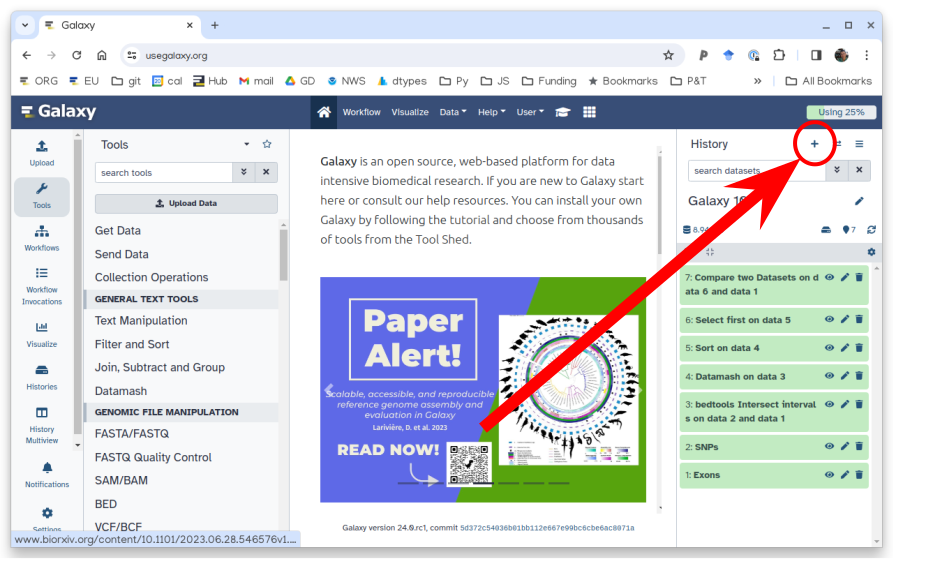
Open image in new tab
 Open image in new tab
 Open image in new tab
 Open image in new tab