Performing experiments in replicates is a cornerstone of modern biological science. However, when integrating data from multiple single-cell sequencing experiments, technical confounders might impact the results.
To reduce technical confounders, such as different experimenters, experimental protocols, sequencing lanes or sequencing technologies, batch correction is often beneficial.
In this tutorial, we will perform batch correction on five datasets of Single-cell Assay for Transposase-Accessible Chromatin using sequencing (scATAC-seq) data with the three algorithms Harmony (Korsunsky et al. 2019), Scanorama (Hie et al. 2019) and the mutual nearest neighbor-based (Haghverdi et al. 2018) algorithm MNC-correct (Zhang et al. 2024). The scATAC-seq analysis will be performed with the tool suite SnapATAC2 (Zhang et al. 2024).
Did you know we have a unique Single Cell Omics Lab with all our single cell tools highlighted to make it easier to use on Galaxy? We recommend this site for all your single cell analysis needs, particularly for newer users.
The Single Cell Omics Lab is a different view of the underlying Galaxy server that organises tools and resources better for single-cell users! It also provides a platform for communities to engage and connect; distribute more targeted news and events; and highlight community-specific funding sources.
Tools are frequently updated to new versions. Your Galaxy may have multiple versions of the same tool available. By default, you will be shown the latest version of the tool. This may NOT be the same tool used in the tutorial you are accessing. Furthermore, if you use a newer tool in one step, and try using an older tool in the next step… this may fail! To ensure you use the same tool versions of a given tutorial, use the Tutorial mode feature.
Open your Galaxy server
Click on the curriculum icon on the top menu, this will open the GTN inside Galaxy.
Navigate to your tutorial
Tool names in tutorials will be blue buttons that open the correct tool for you
Note: this does not work for all tutorials (yet)
You can click anywhere in the grey-ed out area outside of the tutorial box to return back to the Galaxy analytical interface
Warning: Not all browsers work!
We’ve had some issues with Tutorial mode on Safari for Mac users.
Try a different browser if you aren’t seeing the button.
The data analysis is performed with the same tools shown in the tutorial Single-cell ATAC-seq standard processing with SnapATAC2.
That tutorial also explains the steps of the ATAC-seq analysis with SnapATAC2 in more detail.
We recommend completing that tutorial before continuing with batch correction using SnapATAC2.
In this tutorial we will analyze colon samples from multiple donors, provided by the SnapATAC2 documentation. The chrom_sizes file and the gene_annotation file are identical to the previous tutorial Single-cell ATAC-seq standard processing with SnapATAC2.
The five colon_multisample files have been generated by the Cell Ranger ATAC 2.0.0 pipeline from 10X to generate a Fragments File.
A chromosome sizes file can be generated using the tool Compute sequence length ( Galaxy version 1.0.3).
The reference genome can either be selected from cached genomes or uploaded to the galaxy history.
First, we will import the datasets into Galaxy. Next, we will organize all colon_multisample datasets into a collection. Using collections helps streamline the workflow, making the subsequent analysis steps more efficient.
Datasets versus collections
In Galaxy’s history datasets can be present as individual entries or they can be combined into Collections. Why do we need collections? Collections combine multiple individual datasets into a single entity which is easy to manage. Galaxy tools can use collections directly as inputs. Collection can be simple or nested.
Simple collections
Imagine that you’ve uploaded a hundred FASTQ files corresponding to a hundred samples. These will appear as a hundred individual datasets in your history making it very long. But the chances are that when you analyze these data you will do the same thing on each dataset.
To simplify this process you can combine all hundred datasets into a single entity called a dataset collection (or simply a collection or a list). It will appear as a single box in your history making it much easier to understand. Galaxy tools are designed to take collections as inputs. So, for example, if you want to map each of these datasets against a reference genome using, say, Minimap2, you will need to provide minmap2 with just one input, the collection, and it will automatically start 100 jobs behind the scenes and will combine all outputs into a single collection containing BAM files.
There is a number of situations when simple collections are not sufficient to reflect the complexity of the data. To deal with this situation Galaxy allows for nested collections.
Nested collections
Probably the most common example of this is paired end data when each sample is represented by two files: one containing forward reads and another containing reverse reads. In Galaxy you can create nested collection that reflects the hierarchy of the data. In the case of paired data Galaxy supports paired collections.
Get data
Hands On: Data Upload
Create a new history for this tutorial
Import the files from Zenodo or from
the shared data library
Click galaxy-uploadUpload at the top of the activity panel
Select galaxy-wf-editPaste/Fetch Data
Paste the link(s) into the text field
Press Start
Close the window
As an alternative to uploading the data from a URL or your computer, the files may also have been made available from a shared data library:
Go into Libraries (left panel)
Navigate to the correct folder as indicated by your instructor.
On most Galaxies tutorial data will be provided in a folder named GTN - Material –> Topic Name -> Tutorial Name.
Select the desired files
Click on Add to Historygalaxy-dropdown near the top and select as Datasets from the dropdown menu
In the pop-up window, choose
“Select history”: the history you want to import the data to (or create a new one)
Click on Import
Warning: Large file sizes!
The colon_multisample datasets are quite large. The entire tutorial requires approximately 50 GB of storage.
To reduce storage you can change the galaxy-gearUpload Configuration to Defer dataset resolution for the upload of the colon_multisample datasets.
This will delete the datasets after the first analysis step and helps in reducing storage.
You can also permanently delete datasets, which are no longer required.
Deleting datasets individually
To delete datasets individually simply click the galaxy-delete button with dataset’s box. That’s it! This action is reversible: datasets can be undeleted.
Deleting datasets in bulk
To delete multiple datasets at once:
Click history-select-multiple icon at the top of the history pane;
Select datasets you want to delete;
Click the dropdown that would appear at the top of the history;
Select “Delete” option.
This action is also reversible: datasets can be undeleted.
Deleting datasets permanentlywarningDanger zone!
Warning: Permanent is ... PERMANENT!
Datasets deleted in this fashion CANNOT be undeleted!
To delete multiple datasets PERMANENTLY:
Click history-select-multiple icon at the top of the history pane;
Select datasets you want to delete;
Click the dropdown that would appear at the top of the history;
Select “Delete (permanently)” option.
Rename the datasets
galaxy-pencilRename the file gencode.v46.annotation.gtf.gz to gene_annotation.gtf.gz
Click on the galaxy-pencilpencil icon for the dataset to edit its attributes
In the central panel, change the Name field
Click the Save button
Check that the datatypes of the colon_multisample files are set to bed
Click on the galaxy-pencilpencil icon for the dataset to edit its attributes
In the central panel, click galaxy-chart-select-dataDatatypes tab on the top
In the galaxy-chart-select-dataAssign Datatype, select bed from “New Type” dropdown
Tip: you can start typing the datatype into the field to filter the dropdown menu
Click the Save button
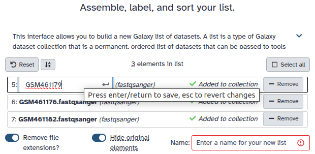
Create a dataset collection with all colon_multisample datasets and rename the collection to Colon Multisample Fragments.
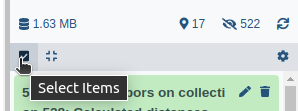
Click on galaxy-selectorSelect Items at the top of the history panel
Check all the datasets in your history you would like to include
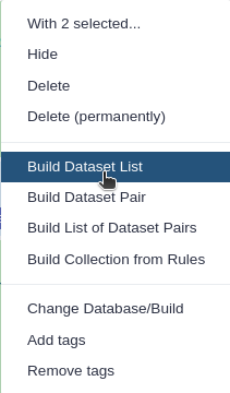
Click n of N selected and choose Advanced Build List
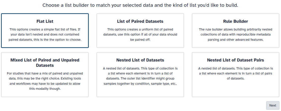
You are in collection building wizard. Choose Flat List and click ‘Next’ button at the right bottom corner.
Double clcik on the file names to edit. For example, remove file extensions or common prefix/suffixes to cleanup the names.
Enter a name for your collection to Colon Multisample Fragments
Click Build to build your collection
Click on the checkmark icon at the top of your history again
SnapATAC2 preprocessing and filtering
With our data imported and the collection assembled, we can now begin the scATAC-seq data preprocessing with SnapATAC2.
The first step is to import the datasets into an AnnData object using the pp.import_data tool. Next, the transcription start site enrichment (TSSe) will be calculated, serving as a quality control (QC) metric to selectively filter droplets containing high-quality cells.
The AnnData format was initially developed for the Scanpy package and is now a widely accepted data format to store annotated data matrices in a space-efficient manner.
Figure 1: AnnData format stores a count matrix `X` together with annotations of observations (i.e., cells) `obs`, variables (i.e., genes) `var`, and unstructured annotations `uns`.
Hands On: Preprocessing and QC
SnapATAC2 Preprocessing ( Galaxy version 2.6.4+galaxy1) with the following parameters:
“Method used for preprocessing”: Import data fragment files and compute basic QC metrics, using 'pp.import_data'
param-collection“Fragment file, optionally compressed with gzip or zstd”: Colon Multisample Fragments (Input dataset collection)
Figure 2: Examplary plots of TSSe from colon_multisample_01 and colon_multisample_02
High-quality cells can be identified in the plot of TSSe scores against a number of unique fragments for each cell.
Question
Where are high-quality cells typically located on a TSSe plot?
Based on these plots, how should the filtering threshold be set?
The cells in the upper right are high-quality cells, enriched for transcription start sites (TSS). Fragments in the lower left represent low-quality cells or empty droplets and should be filtered out.
Setting the minimum TSSe to 7.0 will filter out the lowest quality droplets without loosing too much data.
Filtering the count matrices
The TSSe threshold balances data retention and quality control. In our dataset, the TSSe distributions indicate substantial differences in sample quality between batches. To retain as much biological data as possible, we will use a broader filter (e.g., minimum TSSe = 7.0).
Standard TSSe Thresholds
Strict (TSSe ≥ 10–15): High-confidence cells.
Moderate (TSSe ≥ 7–10): Balances data retention and quality but may include lower-quality cells.
Broad (TSSe ≥ 5–7): Maximizes retention but increases the risk of including lower-quality data.
Choosing the Right Cutoff
If sample quality varies, a moderate threshold (≥7.0) helps retain more data.
If high-quality data is required, stricter filtering (≥10.0) is recommended.
Inspect TSSe distributions to determine the most suitable threshold for your dataset.
Hands On: Filtering
SnapATAC2 Preprocessing ( Galaxy version 2.6.4+galaxy1) with the following parameters:
“Method used for preprocessing”: Filter cell outliers based on counts and numbers of genes expressed, using 'pp.filter_cells'
param-collection“Annotated data matrix”: Colon Multisample AnnDatas TSSe (output of metrics.tssetool)
“Minimum TSS enrichemnt score required for a cell to pass filtering”: 7.0
SnapATAC2 Preprocessing ( Galaxy version 2.6.4+galaxy1) with the following parameters:
“Method used for preprocessing”: Generate cell by bin count matrix, using 'pp.add_tile_matrix'
param-collection“Annotated data matrix”: Colon Multisample AnnDatas filtered (output of pp.filter_cellstool)
“The size of consecutive genomic regions used to record the counts”: 5000
SnapATAC2 Preprocessing ( Galaxy version 2.6.4+galaxy1) with the following parameters:
“Method used for preprocessing”: Perform feature selection, using 'pp.select_features'
param-collection“Annotated data matrix”: Colon Multisample AnnDatas tile_matrix (output of pp.add_tile_matrixtool)
“Number of features to keep”: 50000
pp.add_tile_matrix divides the genome into a specified number of bins, depending on the bin size (f.ex. 5000bp). For each bin, the ATAC-seq reads of individual cells are checked to determine if a read is located in the bin. This is counted as a feature and stored under n_vars in the AnnData object.
Increasing the bin size greatly reduces compute time at the cost of some biological data.
For this reason, the bin size 5000bp has been selected for the colon datasets. In the previous tutorial, the lower bin size of 500bp was chosen, since fewer cells were analyzed.
pp.select_features uses the previously identified features to select the most accessible features for further analysis.
The parameter “Number of features to keep” determines the upper limit of features which can be selected.
Similarly to the bin_size, the Number of Features to keep can also impact downstream clustering. This was demonstrated in the previous tutorial.
SnapATAC2 Preprocessing ( Galaxy version 2.6.4+galaxy1) with the following parameters:
“Method used for preprocessing”: Compute probability of being a doublet using the scrublet algorithm, using 'pp.scrublet'
param-collection“Annotated data matrix”: Colon Multisample AnnDatas features (output of pp.select_featurestool)
SnapATAC2 Preprocessing ( Galaxy version 2.6.4+galaxy1) with the following parameters:
“Method used for preprocessing”: Remove doublets according to the doublet probability or doublet score, using 'pp.filter_doublets'
param-file“Annotated data matrix”: Colon Multisample AnnDatas scrublet (output of pp.scrublettool)
Concatenate the Collection
Before we can continue with the analysis and batch correction, we need to extract the datasets out of the collection and merge them into a single AnnData object.
Extracting datasets from a collection
This is achieved in two steps:
The first dataset is extracted from the collection using Extract dataset
Afterwards, the first dataset will be removed from the collection. This is done by extracting element identifiers and filtering the collection with the name of the first dataset.
Comment:
It is also possible to manually remove a dataset from a collection.
However, manually removing datasets can not be implemented in Galaxy workflows. In contrast the automatic method, shown here, can be represented in a workflow and is therefore much better scalable.
Hands On: Extract datasets
Extract element from collection with the following parameters:
param-collection“Input List”: Colon Multisample AnnDatas filtered_doublets (output of pp.filter_doubletstool)
“How should a dataset be selected?”: The first dataset
Extract element identifiers ( Galaxy version 0.0.2) with the following parameters:
param-collection“Dataset collection”: Colon Multisample AnnDatas filtered_doublets (output of pp.filter_doubletstool)
Select first with the following parameters:
“Select first”: 1
param-file“from”: Element identifiers (output of Extract element identifierstool)
Filter collection with the following parameters:
param-collection“Input Collection”: Colon Multisample AnnDatas filtered_doublets (output of pp.filter_doubletstool)
“How should the elements to remove be determined?”: Remove if identifiers are PRESENT in file
param-file“Filter out identifiers present in”: select_first (output of Select firsttool)
galaxy-pencil Rename the filtered collection to Colon Multisample 02-05
Concatenating all AnnData files
Hands On: Concatenate
Manipulate AnnData ( Galaxy version 0.10.3+galaxy0) with the following parameters:
param-file“Annotated data matrix”: colon_multisample_01 (output of Extract datasettool)
“Function to manipulate the object”: Concatenate along the observations axis
param-collection“Annotated data matrix to add”: Colon Multisample 02-05 (output of Filter collectiontool)
“Join method”: Intersection of variables
“Key to add the batch annotation to obs”: batch
The runtime of this operation depends on the dataset size. For colon_multisample datasets, concatenation may take up to 1 hour.
For larger datasets, the tool’s allocated memory may be insufficient, causing the operation to fail. In that case, you will see the following error message:
Fatal error: Exit code 137 ()
In this case, report the issue so that administrators can increase the memory limit, allowing the job to complete successfully.
Writing bug reports is a good skill to have as bioinformaticians, and a key point is that you should include enough information from the first message to help the process of resolving your issue more efficient and a better experience for everyone.
What to include
Which commands did you run, precisely, we want details. Which flags did you set?
Which server(s) did you run those commands on?
What account/username did you use?
Where did it go wrong?
What were the stdout/stderr of the tool that failed? Include the text.
Did you try any workarounds? What results did those produce?
(If relevant) screenshot(s) that show exactly the problem, if it cannot be described in text. Is there a details panel you could include too?
If there are job IDs, please include them as text so administrators don’t have to manually transcribe the job ID in your picture.
It makes the process of answering ‘bug reports’ much smoother for us, as we will have to ask you these questions anyway. If you provide this information from the start, we can get straight to answering your question!
What does a GOOD bug report look like?
The people who provide support for Galaxy are largely volunteers in this community, so try and provide as much information up front to avoid wasting their time:
I encountered an issue: I was working on (this server> and trying to run (tool)+(version number) but all of the output files were empty. My username is jane-doe.
Here is everything that I know:
The dataset is green, the job did not fail
This is the standard output/error of the tool that I found in the information page (insert it here)
I have read it but I do not understand what X/Y means.
The job ID from the output information page is 123123abdef.
I tried re-running the job and changing parameter Z but it did not change the result.
Could you help me?
galaxy-pencil Rename the AnnData output to Multisample AnnData
galaxy-eye Inspect the general information of Multisample AnnData
Many toolsets producing outputs in AnnData formats in Galaxy, provide the general information by default:
Click on the name of the dataset in the history to expand it. The general Anndata information will be given in the expanded box.
Alternatively, expand the dataset and click on detailsDataset Details. Scroll to Job Information and inspect the Tool Standard Output.
If a tool does not provide general AnnData information or a more specific query is needed, you can use Inspect AnnData ( Galaxy version 0.10.3+galaxy0).
How many colon cells are present in this AnnData object?
What does the ‘batch’ annotation indicate?
What do the ‘count-‘ and ‘selected-‘ annotations represent?
There are 34,372 cells.
The ‘batch’ annotation labels cells according to their sample number (0–4). This annotation will later be used by batch correction algorithms to generate clusters from multiple samples.
‘count’ and ‘selected’ are variable annotations representing detected and selected features. The sample number (0–4) indicates the dataset that generated these annotations.
Dimension Reduction
Now that all samples have been concatenated into a single AnnData object, the most accessible features of the combined count matrix must be selected. The previously chosen features were sample-specific and cannot be used for dimensionality reduction. Therefore, the most accessible features will be reselected, followed by dimensionality reduction using matrix-free spectral embedding.
Hands On: Spectral Embedding
SnapATAC2 Preprocessing ( Galaxy version 2.6.4+galaxy1) with the following parameters:
“Method used for preprocessing”: Perform feature selection, using 'pp.select_features'
param-file“Annotated data matrix”: Multisample AnnData (output of Manipulate AnnDatatool)
“Number of features to keep”: 50000
SnapATAC2 Clustering ( Galaxy version 2.6.4+galaxy1) with the following parameters:
“Dimension reduction and clustering”: Perform dimensionality reduction using Laplacian Eigenmap ('tl.spectral')
param-file“Annotated data matrix”: Multisample AnnData features (output of pp.select_featurestool)
“Distance metric”: cosine
galaxy-pencil Rename the output AnnData object to Multisample AnnData spectral
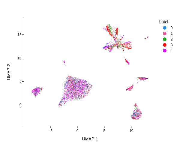
Control Without Batch Correction
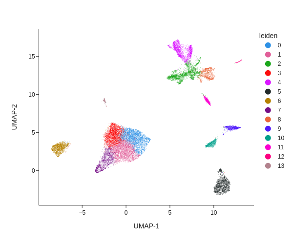
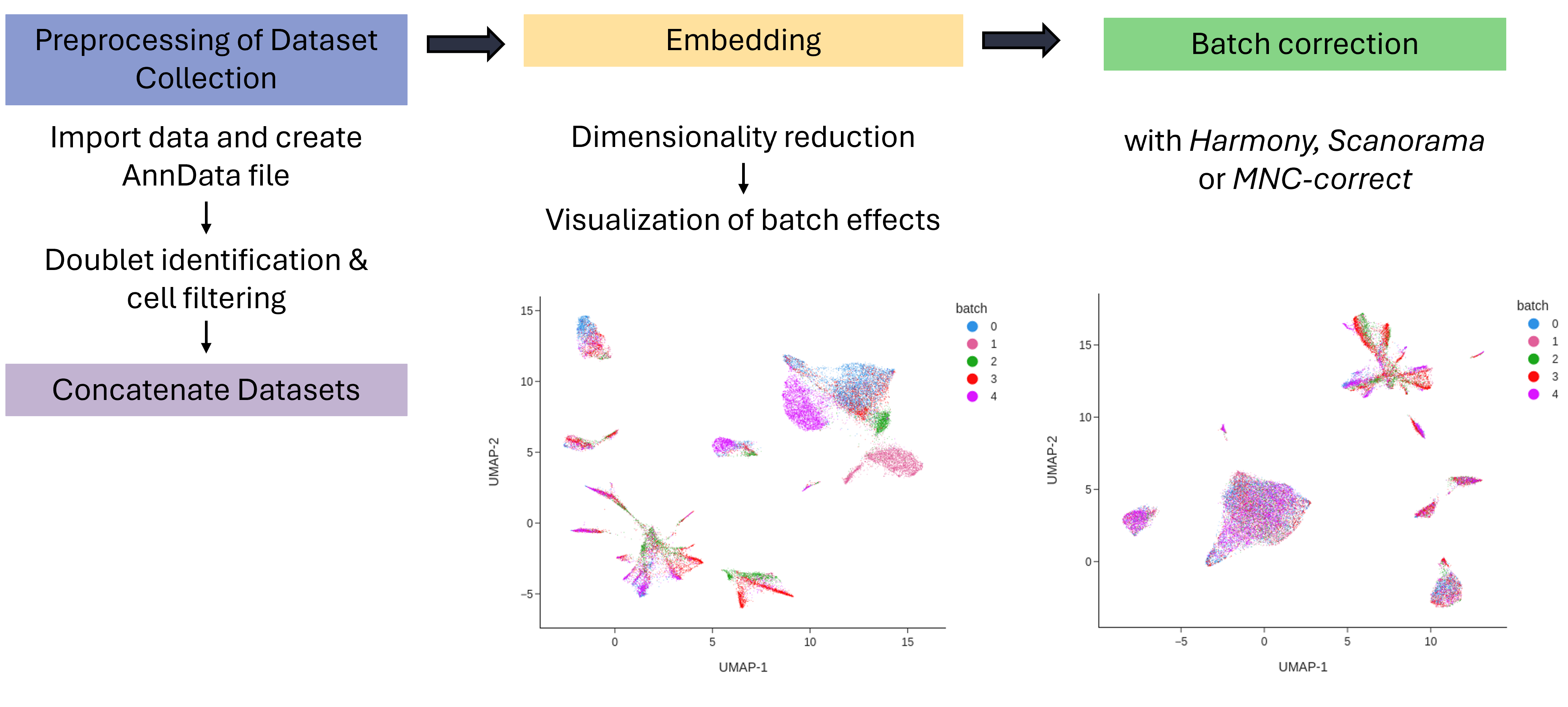
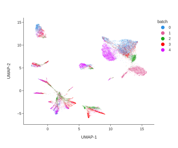
Batch effects can be visualized using a Uniform Manifold Approximation and Projection (UMAP) projection, where samples are colored by their batch annotation (obs: 'batch').
Hands On: UMAP Projection Without Batch Correction
SnapATAC2 Clustering ( Galaxy version 2.6.4+galaxy1) with the following parameters:
“Dimension reduction and Clustering”: Compute UMAP using 'tl.umap'
param-file“Annotated data matrix”: Multisample AnnData spectral (output of tl.spectraltool)
galaxy-pencil Rename the output AnnData object to Multisample AnnData UMAP.
SnapATAC2 Plotting ( Galaxy version 2.6.4+galaxy1) with the following parameters:
“Method used for plotting”: Plot the UMAP embedding using 'pl.umap'
param-file“Annotated data matrix”: Multisample AnnData UMAP (output of tl.umaptool)
“Color”: batch
“Height of the plot”: 500
galaxy-pencil Rename the generated image to spectral-UMAP-No Batch Correction.
galaxy-eye Inspect the .png output.
Question
How do batch effects appear in this plot?
What would a plot without batch effects look like?
Batch effects appear as distinct clusters where samples are unevenly distributed. For example, in the upper right corner, each batch forms a separate group. These differences are likely technical artifacts rather than true biological variation.
A plot without batch effects would show cells from all samples evenly mixed, with no distinct clusters corresponding to individual batches.
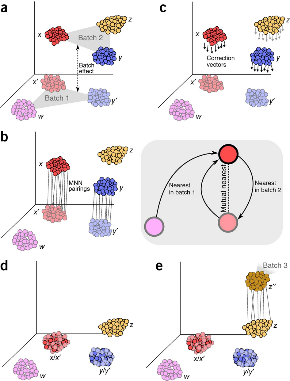
Batch correction
After confirming the presence of batch effects, they should be removed using correction algorithms. SnapATAC2 provides three batch correction methods: Harmony, MNC-correct, and Scanorama. To determine the most suitable algorithm for your dataset, compare the outputs of each method.
Batch correction algorithms adjust the cell-by-feature count matrix to account for batch-specific differences between samples.
Batch effects can arise from various technical sources, such as sequencing lanes, plates, protocols, and handling. Additionally, biological factors, including tissue types, species, and inter-individual variation, can also contribute to batch effects Luecken et al. 2021.
Many batch correction algorithms have been developed, with most scATAC-seq methods adapted from scRNA-seq batch removal techniques.
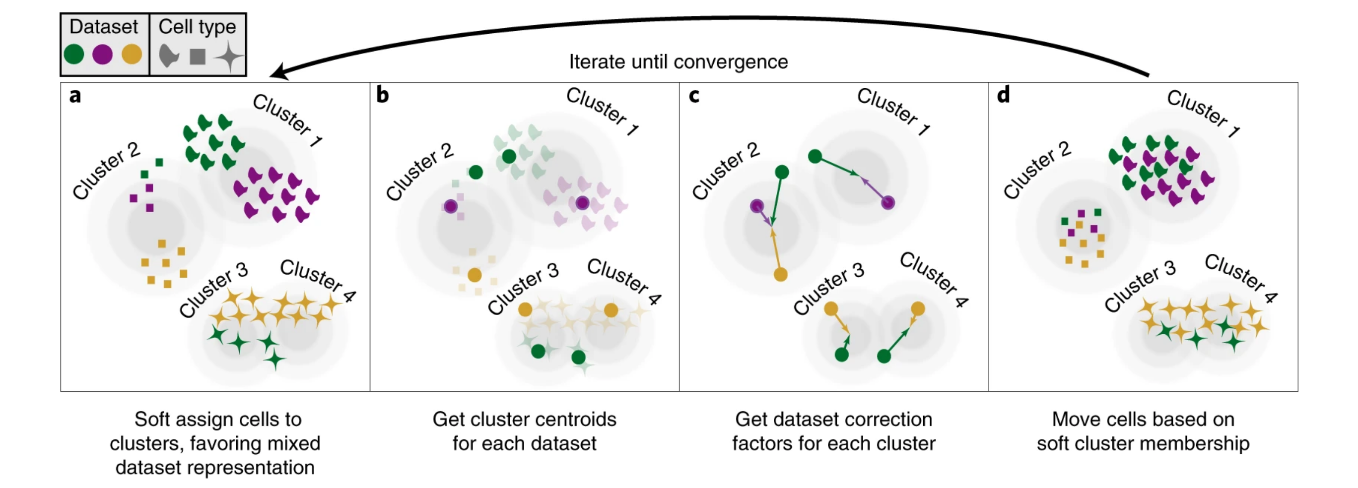
HarmonyKorsunsky et al. 2019 is a principal component analysis (PCA)-based method that leverages lower-dimensional data to assign cells to new clusters. It prioritizes multi-sample clustering to integrate datasets by computing linear correction factors for each batch and cluster, iteratively adjusting cell positions until optimal batch correction is achieved.
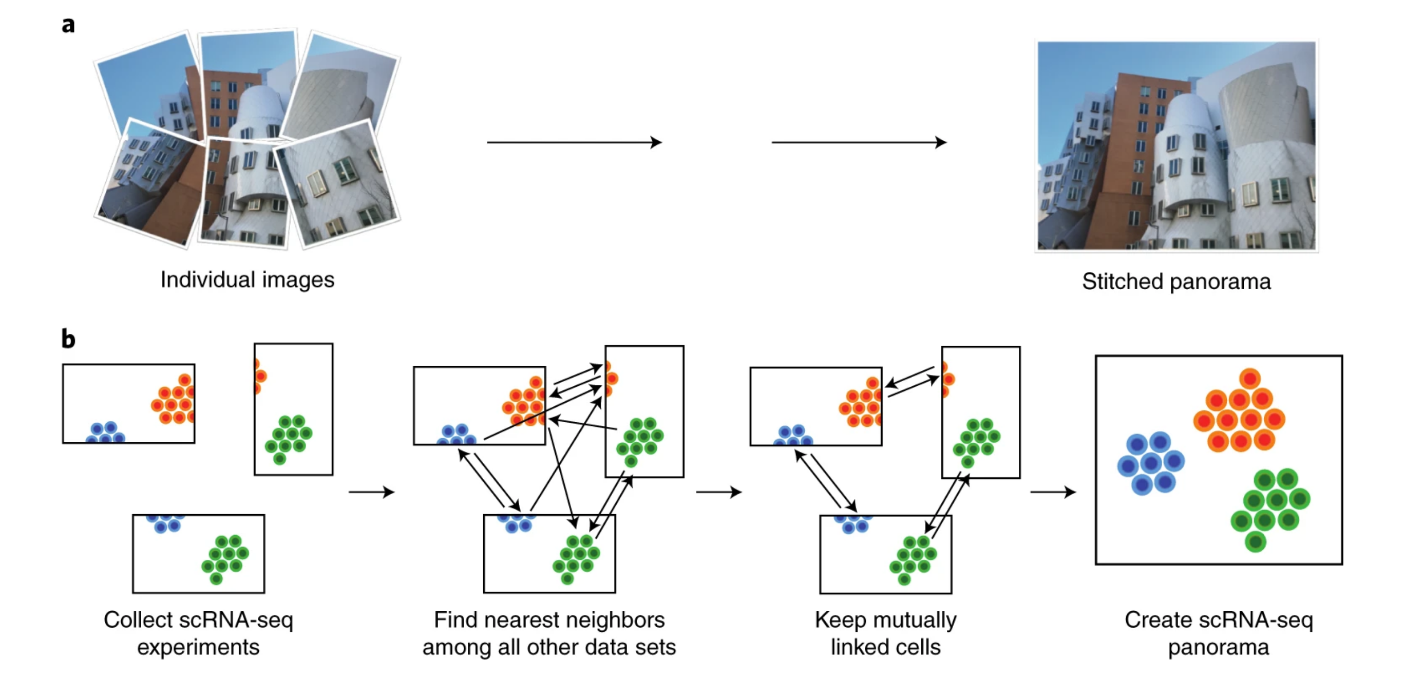
ScanoramaHie et al. 2019 performs panorama stiching, to find and merge overlapping cell types.
MNC-correctZhang et al. 2024 is a modified version of the mutual nearest neighbor algorithm Haghverdi et al. 2018. It calculates centroids for batch-specific clusters and identifies pairs of mutual nearest centroids (MNC) across batches. Correction vectors then align the batches in the same plane. Additionally, MNC-correct can be run iteratively to refine corrections for optimal alignment.
We will first use Harmony to correct batch effects, followed by testing the other methods.
Hands On: Batch correction and visualization
SnapATAC2 Preprocessing ( Galaxy version 2.6.4+galaxy1) with the following parameters:
“Method used for preprocessing”: Use harmonypy to integrate different experiments,using 'pp.harmony'
param-file“Annotated data matrix”: Multisample AnnData UMAP (output of tl.umaptool)
SnapATAC2 Clustering ( Galaxy version 2.6.4+galaxy1) with the following parameters:
“Dimension reduction and Clustering”: Compute Umap, using 'tl.umap'
param-file“Annotated data matrix”: Multisample AnnData harmony (output of pp.harmonytool)
“Use the indicated representation in .obsm“: X_spectral_harmony
“adata.obs key under which t add cluster labels”: umap_harmony
galaxy-pencil Rename the AnnData output to Multisample AnnData harmony UMAP
Comment: Key for Cluster Labels
Adding the new UMAP embeddings under the key umap_harmony preserves the non-batch-corrected embeddings in the AnnData object.
Alternatively, leaving this parameter empty will overwrite the existing embeddings.
SnapATAC2 Plotting ( Galaxy version 2.6.4+galaxy1) with the following parameters:
“Method used for plotting”: Plot the UMAP embedding, using 'pl.umap'
param-file“Annotated data matrix”: Multisample AnnData harmony UMAP (output of tl.umaptool)
“Color”: batch
“Use the indicated representation in .obsm”: X_umap_harmony
“Height of the plot”: 500
galaxy-pencil Rename the generated image to spectral-UMAP-harmony
galaxy-eye Inspect the .png output
Question
How did Harmony affect the appearance of this plot?
Are there areas in the plot where batch effects persist?
Harmony has successfully removed most batch effects. Notably, the center-left groups have merged into a single larger group containing all batches.
Yes, some batch effects remain, particularly in the upper-right corner, where batch-specific colors do not fully overlap. However, this could also be due to certain samples having fewer cells, leading to underrepresentation in clusters of rare cell types. Therefore, it is unclear whether Harmony has completely eliminated all batch effects.
Other batch correction methods can be applied using SnapATAC2 Preprocessing ( Galaxy version 2.6.4+galaxy1), including pp.mnc_correct and pp.scanorama_integrate.
For MNC-correct, the number of iterations can be adjusted.
To determine the optimal batch correction method, it is recommended to test different algorithms and parameter settings.
Example outputs from Scanorama and MNC-correct are shown below:
Figure 3: UMAP plots of batch correction with different methods. (a) Batch correction with MNC-correct and default settings. (b) Batch correction with Scanorama. (c) Batch correction with MNC-correct and 30 iterations.
Question
Compare these plots with the output of Harmony. Which algorithm is best-suited for the colon datasets?
Harmony achieved the best batch integration, as it produced the fewest single-batch groups. Scanorama and MNC-correct (with default settings) did not integrate the batches as effectively. However, MNC-correct with 30 iterations significantly reduced batch effects and could also be used for further analysis.
Clustering of the batch corrected samples
The analysis can now continue using the same methods outlined in the standard pathway. The batch-corrected embeddings are clustered and visualized using the Leiden algorithm.
Hands On: Leiden clustering and visualization
SnapATAC2 Clustering ( Galaxy version 2.6.4+galaxy1) with the following parameters:
“Dimension reduction and Clustering”: Compute a neighborhood graph of observations, using 'pp.knn'
param-file“Annotated data matrix”: Multisample AnnData harmony UMAP (output of tl.umaptool)
“The key for the matrix”: X_spectral_harmony
Each batch correction algorithm stores its corrected matrix under a specific key:
Harmony: X_spectral_harmony
MNC-correct: X_spectral_mnn
Scanorama: X_spectral_scanorama
These keys are stored in the AnnData object under 'obsm'.
SnapATAC2 Clustering ( Galaxy version 2.6.4+galaxy1) with the following parameters:
“Dimension reduction and Clustering”: Cluster cells into subgroups, using 'tl.leiden'
param-file“Annotated data matrix”: Multisample AnnData harmony knn (output of pp.knntool)
“Whether to use the Constant Potts Model (CPM) or modularity”: modularity
galaxy-pencil Rename the AnnData output to Multisample AnnData harmony leiden
SnapATAC2 Plotting ( Galaxy version 2.6.4+galaxy1) with the following parameters:
“Method used for plotting”: Plot the UMAP embedding, using 'pl.umap'
param-file“Annotated data matrix”: anndata_out (output of tl.leidentool)
“Color”: leiden
“Use the indicated representation in .obsm”: X_umap_harmony
“Height of the plot”: 500
galaxy-pencil Rename the generated image to spectral-UMAP-harmony-leiden
galaxy-eye Inspect the .png output
After integrating the datasets and clustering the cells, the scATAC-seq analysis can proceed with downstream analysis. This includes cell cluster annotation and differential peak analysis.
Comment
The SnapATAC2 tools for differential peak analysis are available in Galaxy, but no GTN training materials are currently provided. Until a tutorial is available, you can refer to the SnapATAC2 documentation for a tutorial on differential peak analysis.
The tools are available in Galaxy under SnapATAC2 Peaks and Motif ( Galaxy version 2.6.4+galaxy1).
Conclusion
congratulations Well done, you’ve made it to the end! You might want to consult your results with this control history, or check out the full workflow for this tutorial.
In this tutorial, we integrated five scATAC-seq colon samples using a scalable Galaxy workflow. We compared different batch integration algorithms to identify the most suitable method for our data. Finally, we clustered the cells to prepare the data for downstream analysis.
You've Finished the Tutorial
Please also consider filling out the Feedback Form as well!
Key points
Batch correction is important for the integration of data from multiple experiments
Batch correction algorithms identify similar cells and move them closer together through appropriate correction vectors.
Frequently Asked Questions
Have questions about this tutorial? Have a look at the available FAQ pages and support channels
Further information, including links to documentation and original publications, regarding the tools, analysis techniques and the interpretation of results described in this tutorial can be found here.
References
Haghverdi, L., A. T. L. Lun, M. D. Morgan, and J. C. Marioni, 2018 Batch effects in single-cell RNA-sequencing data are corrected by matching mutual nearest neighbors. Nature Biotechnology 36: 421–427. 10.1038/nbt.4091
Hie, B., B. Bryson, and B. Berger, 2019 Efficient integration of heterogeneous single-cell transcriptomes using Scanorama. Nature Biotechnology 37: 685–691. 10.1038/s41587-019-0113-3
Korsunsky, I., N. Millard, J. Fan, K. Slowikowski, F. Zhang et al., 2019 Fast, sensitive and accurate integration of single-cell data with Harmony. Nature Methods 16: 1289–1296. 10.1038/s41592-019-0619-0
Luecken, M. D., M. Büttner, K. Chaichoompu, A. Danese, M. Interlandi et al., 2021 Benchmarking atlas-level data integration in single-cell genomics. Nature Methods 19: 41–50. 10.1038/s41592-021-01336-8
Zhang, K., N. R. Zemke, E. J. Armand, and B. Ren, 2024 A fast, scalable and versatile tool for analysis of single-cell omics data. Nature Methods 21: 217–227. 10.1038/s41592-023-02139-9
Glossary
QC
quality control
TSS
transcription start sites
TSSe
transcription start site enrichment
UMAP
Uniform Manifold Approximation and Projection
scATAC-seq
Single-cell Assay for Transposase-Accessible Chromatin using sequencing
Feedback
Did you use this material as an instructor? Feel free to give us feedback on how it went.
Did you use this material as a learner or student? Click the form below to leave feedback.
Hiltemann, Saskia, Rasche, Helena et al., 2023 Galaxy Training: A Powerful Framework for Teaching! PLOS Computational Biology 10.1371/journal.pcbi.1010752
Batut et al., 2018 Community-Driven Data Analysis Training for Biology Cell Systems 10.1016/j.cels.2018.05.012
@misc{single-cell-scatac-batch-correction-snapatac2,
author = "Timon Schlegel",
	title = "Multi-sample batch correction with Harmony and SnapATAC2 (Galaxy Training Materials)",
	year = "",
	month = "",
	day = "",
	url = "\url{https://training.galaxyproject.org/training-material/topics/single-cell/tutorials/scatac-batch-correction-snapatac2/tutorial.html}",
	note = "[Online; accessed TODAY]"
}
@article{Hiltemann_2023,
	doi = {10.1371/journal.pcbi.1010752},
	url = {https://doi.org/10.1371%2Fjournal.pcbi.1010752},
	year = 2023,
	month = {jan},
	publisher = {Public Library of Science ({PLoS})},
	volume = {19},
	number = {1},
	pages = {e1010752},
	author = {Saskia Hiltemann and Helena Rasche and Simon Gladman and Hans-Rudolf Hotz and Delphine Larivi{\`{e}}re and Daniel Blankenberg and Pratik D. Jagtap and Thomas Wollmann and Anthony Bretaudeau and Nadia Gou{\'{e}} and Timothy J. Griffin and Coline Royaux and Yvan Le Bras and Subina Mehta and Anna Syme and Frederik Coppens and Bert Droesbeke and Nicola Soranzo and Wendi Bacon and Fotis Psomopoulos and Crist{\'{o}}bal Gallardo-Alba and John Davis and Melanie Christine Föll and Matthias Fahrner and Maria A. Doyle and Beatriz Serrano-Solano and Anne Claire Fouilloux and Peter van Heusden and Wolfgang Maier and Dave Clements and Florian Heyl and Björn Grüning and B{\'{e}}r{\'{e}}nice Batut and},
	editor = {Francis Ouellette},
	title = {Galaxy Training: A powerful framework for teaching!},
	journal = {PLoS Comput Biol}
}
Funding
These individuals or organisations provided funding support for the development of this resource
Questions:


Open image in new tab
Open image in new tab
Open image in new tab