Phylodiversity analysis quick tutorial
| Author(s) |
|
| Reviewers |
|
OverviewQuestions:
Objectives:
How to use the phylodiversity workflow?
How to construct phyloregions from occurrences species data, phylogenic data and geograpics data?
Requirements:
Learning how to use the phylodiversity workflow.
Compute endemism index
Create a phyloregion map
Time estimation: 2 hoursSupporting Materials:Published: Jun 6, 2025Last modification: May 7, 2026License: Tutorial Content is licensed under Creative Commons Attribution 4.0 International License. The GTN Framework is licensed under MITpurl PURL: https://gxy.io/GTN:T00538version Revision: 2
This tutorial is designed to guide you through the Phylodiversity Galaxy workflow, demonstrating how to easily compute phylodiversity and create phyloregions from phylogeny, occupency and spatial files.
The tutorial will provide a detailed explanation of inputs, workflow steps, and outputs. This tutorial gives a practical example, highlighting a use case extract from souhtern sea actinos populations.
The primary goal of this workflow is to compute phylodiversity index and identify phyloregions. The project’s objective is to offer accessible, reproducible and transparents solutions for analyse phylodiversity.
This workflow is composed of four tools:
- PhylOccuMatcher
- CRSConverter
- PhyloIndex
- EstimEndem
In this tutorial, we estimate your data are correctly formated.
AgendaIn this tutorial, we will cover:
Before starting
This part will present the type of data you need to run the ecoregionalization workflow. This data will be downloaded in the next part of the tutorial.
phylogenic tree file
The first file needed for this workflow is the phylogenetic tree of your interested species. In this example it’a a simplified phylogeny of the actinopterigy This file must be at newick format.
occupancy file
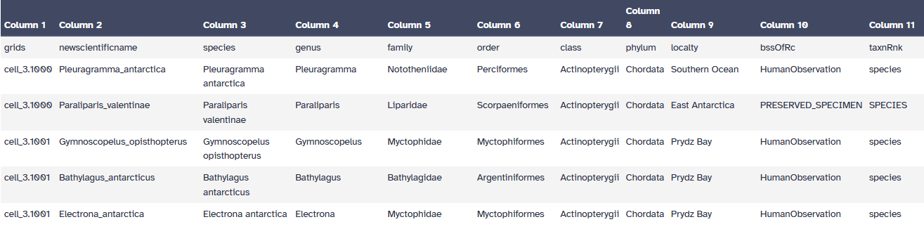
The second file is an occupancy file, each line is a species, the decimal separator must be “.” and the column must be separated with “\t”(={Tabulation}). You need to have a column “grids” containing the cell of the grid you’ve seen your species and the name of the column with the species names must be “newscientificname”.
| grids | newscientificname | … | … | … |
|---|---|---|---|---|
| ——- | ——————- | ——- | —– | … |
| … | … | … | … | … |
Shapefile
The last file is a spatial file in shapefile format. In Galaxy this type of file must be uploaded as a composite file of type shp. This kind of file must have at least 3 file with the same name and 3 different extension : .shp, .shx end .dbf. you can have more file optionally like the .prj file.
Get data
Hands On: Data Upload
- Create a new history for this tutorial
Import the files from Zenodo or from the shared data library (
GTN - Material->ecology->Phylodiversity analysis quick tutorial):For the
tabularandnewickdatafileshttps://zenodo.org/records/15601932/files/phylogeny_test https://zenodo.org/records/15601932/files/grid_test.tabularFor the composite
shpdatafile (you here need to download locally each file to upload it from the “Composite” menu of “Upload Files” tool, selectingshpdatatype)https://zenodo.org/records/15601932/files/shapefile.dbf https://zenodo.org/records/15601932/files/shapefile.prj https://zenodo.org/records/15601932/files/shapefile.shx https://zenodo.org/records/15601932/files/shapefile.shp
- Copy the link location
Click galaxy-upload Upload at the top of the activity panel
- Select galaxy-wf-edit Paste/Fetch Data
Paste the link(s) into the text field
Press Start
- Close the window
As an alternative to uploading the data from a URL or your computer, the files may also have been made available from a shared data library:
- Go into Libraries (left panel)
- Navigate to the correct folder as indicated by your instructor.
- On most Galaxies tutorial data will be provided in a folder named GTN - Material –> Topic Name -> Tutorial Name.
- Select the desired files
- Click on Add to History galaxy-dropdown near the top and select as Datasets from the dropdown menu
In the pop-up window, choose
- “Select history”: the history you want to import the data to (or create a new one)
- Click on Import
- Rename the datasets
Check that the datatype of the phylogenic file is
newick(often not automatically detected to this format butjson), occupancy filetabularand the spatial file a composite dataset of typeshapefile
- Click on the galaxy-pencil pencil icon for the dataset to edit its attributes
- In the central panel, click galaxy-chart-select-data Datatypes tab on the top
- In the galaxy-chart-select-data Assign Datatype, select
newickfrom “New Type” dropdown
- Tip: you can start typing the datatype into the field to filter the dropdown menu
- Click the Save button
A good pratice is also to add to each datafile a tag corresponding for example to the taxon, here
Actinopterygiansor other relevant information.Datasets can be tagged. This simplifies the tracking of datasets across the Galaxy interface. Tags can contain any combination of letters or numbers but cannot contain spaces.
To tag a dataset:
- Click on the dataset to expand it
- Click on Add Tags galaxy-tags
- Add tag text. Tags starting with
#will be automatically propagated to the outputs of tools using this dataset (see below).- Press Enter
- Check that the tag appears below the dataset name
Tags beginning with
#are special!They are called Name tags. The unique feature of these tags is that they propagate: if a dataset is labelled with a name tag, all derivatives (children) of this dataset will automatically inherit this tag (see below). The figure below explains why this is so useful. Consider the following analysis (numbers in parenthesis correspond to dataset numbers in the figure below):
- a set of forward and reverse reads (datasets 1 and 2) is mapped against a reference using Bowtie2 generating dataset 3;
- dataset 3 is used to calculate read coverage using BedTools Genome Coverage separately for
+and-strands. This generates two datasets (4 and 5 for plus and minus, respectively);- datasets 4 and 5 are used as inputs to Macs2 broadCall datasets generating datasets 6 and 8;
- datasets 6 and 8 are intersected with coordinates of genes (dataset 9) using BedTools Intersect generating datasets 10 and 11.
Now consider that this analysis is done without name tags. This is shown on the left side of the figure. It is hard to trace which datasets contain “plus” data versus “minus” data. For example, does dataset 10 contain “plus” data or “minus” data? Probably “minus” but are you sure? In the case of a small history like the one shown here, it is possible to trace this manually but as the size of a history grows it will become very challenging.
The right side of the figure shows exactly the same analysis, but using name tags. When the analysis was conducted datasets 4 and 5 were tagged with
#plusand#minus, respectively. When they were used as inputs to Macs2 resulting datasets 6 and 8 automatically inherited them and so on… As a result it is straightforward to trace both branches (plus and minus) of this analysis.More information is in a dedicated #nametag tutorial.

Data formatting
The first step is to be sure your data are well formated. If all your file are in good format and do have the needed column as specified before, you can move forward.
An example of occupancy file:
 Open image in new tab
Phylodiversity Workflow
Match your phylogeny and occupancy with PhylOccuMatcher
Hands On: run PhylOccuMatcher
- PhylOccuMatcher ( Galaxy version 1.0+galaxy0) with the following parameters:
- param-file “Phylogeny file (Newick format)”:
phylogeny_test(Input dataset)- param-file “Occupancy data (Tabular format)”:
grid_test.tabular(Input dataset)Comment: short descriptionThis tool is the simpliest, you, normally, don’t have anything to change and just have to run it with your file as input.
modifying the projection with CRSconverter
Hands On: run CRSConverter
- CRSconverter ( Galaxy version 1.1+galaxy0) with the following parameters:
- param-file “shapefile”:
composite_dataset(Input dataset)Warning: Pay attention to output formatThis tool provide multiple possible outputs formats but only the shapefile format can be used for the workflow. The other output format are graphical representation for the user to visualize. If you want it you can rerun this tool outside of the workflow withe the same input and option.
Warning: Pay attention to the tool versionFor the workflow to work you need to use the CRSConverter 1.1 not the 1.0. So be cautious it’s the case because if you use the 1.0 version the workflow will crash during the last step.
Comment: short descriptionThe main interest of using this tool is to modify the projection of your shapefile. To use it you’ll have to select the parameter you need in the advanced option before running this tool.
Compute phylodiversity index with PhyloIndex
Hands On: run PhyloIndex
- PhyloIndex ( Galaxy version 1.0+galaxy0) with the following parameters:
- param-file “Phylogeny file (Newick format)”:
Phylogeny with occupancy data(output of PhylOccuMatcher tool)- param-file “Occupancy data (Tabular format)”:
Matched output data(output of PhylOccuMatcher tool)Comment: short descriptionThis tool compute phylodiversity index, It include some randomness so, for reproducibility, you’ll need to select a random seed. Moreover you’ll need to select the way of modeling you want by choosing between 3 propositon: -“tipshuffle”: shuffles tip labels multiple times. -“rowwise”: shuffles sites (i.e., varying richness) and keeping species occurrence frequency constant. -“colwise”: shuffles species occurrence frequency and keeping site richness constant. The default value is the tipshuffle method
Estimate the endemism with EstimEndem
Hands On: run EstimEndem
- EstimEndem ( Galaxy version 0.1.0+galaxy0) with the following parameters:
- param-file “Phylogeny file (Newick format)”:
Phylogeny with occupancy data(output of PhylOccuMatcher tool)- param-file “Occupancy data (Tabular format)”:
Matched output data(output of PhylOccuMatcher tool)- param-file “input_shapefile”:
shapefile(output of CRSconverter tool)Comment: short descriptionThe output of this tool is a shapefile with the clusterisation done in function of the endemism. You’ll have to choose a number of cluster you want and the clustering method you want.
Comment: More tips and infoIf you have no idea how many cluster you want, the tool start with an estimation of how many clusters are optimal between 0 to 30. So you can firstly run the tool with default value and go check the standard output to check the recommanded number. However keep in mind that this estimation is purely statistics and don’t always have biologic reasons.
Conclusion
Congratulation for successfully completed the Phylodiversity workflow. Here is the end of this quick tutorial. Don’t hesitate to contact us if you have any questions or if you have ideas for improvment of this workflow.
You've Finished the Tutorial
Key points
The PhylOccuMatcher tool allows to match phylogeny and occupancy data.
The CRSconverter tool transforms geographical vector data to a specified coordinated system, WGS84 by default. This tool is usefull as a step of a workfow to force the coordinating system needed by futher steps.
Frequently Asked Questions
Have questions about this tutorial? Have a look at the available FAQ pages and support channelsUseful literature
Further information, including links to documentation and original publications, regarding the tools, analysis techniques and the interpretation of results described in this tutorial can be found here.
Feedback
Did you use this material as an instructor? Feel free to give us feedback on how it went.
Did you use this material as a learner or student? Click the form below to leave feedback.

Citing this Tutorial
- Elouan Le Mestric, Yvan Le Bras, Phylodiversity analysis quick tutorial (Galaxy Training Materials). https://training.galaxyproject.org/training-material/topics/ecology/tutorials/phylodiversity_workflow/tutorial.html Online; accessed TODAY
- Hiltemann, Saskia, Rasche, Helena et al., 2023 Galaxy Training: A Powerful Framework for Teaching! PLOS Computational Biology 10.1371/journal.pcbi.1010752
- Batut et al., 2018 Community-Driven Data Analysis Training for Biology Cell Systems 10.1016/j.cels.2018.05.012
@misc{ecology-phylodiversity_workflow,
author = "Elouan Le Mestric and Yvan Le Bras",
	title = "Phylodiversity analysis quick tutorial (Galaxy Training Materials)",
	year = "",
	month = "",
	day = "",
	url = "\url{https://training.galaxyproject.org/training-material/topics/ecology/tutorials/phylodiversity_workflow/tutorial.html}",
	note = "[Online; accessed TODAY]"
}
@article{Hiltemann_2023,
	doi = {10.1371/journal.pcbi.1010752},
	url = {https://doi.org/10.1371%2Fjournal.pcbi.1010752},
	year = 2023,
	month = {jan},
	publisher = {Public Library of Science ({PLoS})},
	volume = {19},
	number = {1},
	pages = {e1010752},
	author = {Saskia Hiltemann and Helena Rasche and Simon Gladman and Hans-Rudolf Hotz and Delphine Larivi{\`{e}}re and Daniel Blankenberg and Pratik D. Jagtap and Thomas Wollmann and Anthony Bretaudeau and Nadia Gou{\'{e}} and Timothy J. Griffin and Coline Royaux and Yvan Le Bras and Subina Mehta and Anna Syme and Frederik Coppens and Bert Droesbeke and Nicola Soranzo and Wendi Bacon and Fotis Psomopoulos and Crist{\'{o}}bal Gallardo-Alba and John Davis and Melanie Christine Föll and Matthias Fahrner and Maria A. Doyle and Beatriz Serrano-Solano and Anne Claire Fouilloux and Peter van Heusden and Wolfgang Maier and Dave Clements and Florian Heyl and Björn Grüning and B{\'{e}}r{\'{e}}nice Batut and},
	editor = {Francis Ouellette},
	title = {Galaxy Training: A powerful framework for teaching!},
	journal = {PLoS Comput Biol}
}
Funding
These individuals or organisations provided funding support for the development of this resource
Congratulations on successfully completing this tutorial!
You can use Ephemeris's
shed-tools installcommand to install the tools used in this tutorial.shed-tools install [-g GALAXY] [-a API_KEY] -t <(curl https://training.galaxyproject.org/training-material/api/topics/ecology/tutorials/phylodiversity_workflow/tutorial.json | jq .admin_install_yaml -r)Alternatively you can copy and paste the following YAML
---
install_tool_dependencies: true
install_repository_dependencies: true
install_resolver_dependencies: true
tools:
- name: crsconverter
  owner: ecology
  revisions: 5da4708809a0
  tool_panel_section_label: Phylodiversity
  tool_shed_url: https://toolshed.g2.bx.psu.edu/
- name: estimate_endem
  owner: ecology
  revisions: b8f366e925e7
  tool_panel_section_label: Phylodiversity
  tool_shed_url: https://toolshed.g2.bx.psu.edu/
- name: phylo_index
  owner: ecology
  revisions: 1d73a4af71f5
  tool_panel_section_label: Phylodiversity
  tool_shed_url: https://toolshed.g2.bx.psu.edu/
- name: phylogenetic_occupancy_matcher
  owner: ecology
  revisions: e260f1a598da
  tool_panel_section_label: Phylodiversity
  tool_shed_url: https://toolshed.g2.bx.psu.edu/