name: inverse layout: true class: center, middle, inverse <div class="my-header"><span> <a href="/training-material/topics/metabolomics" title="Return to topic page" ><i class="fa fa-level-up" aria-hidden="true"></i></a> <a href="https://github.com/galaxyproject/training-material/edit/main/topics/metabolomics/tutorials/lcms-preprocessing/slides.html"><i class="fa fa-pencil" aria-hidden="true"></i></a> </span></div> <div class="my-footer"><span> <img src="/training-material/assets/images/GTN-60px.png" alt="Galaxy Training Network" style="height: 40px;"/> </span></div> --- <img src="/training-material/assets/images/GTNLogo1000.png" alt="Galaxy Training Network" class="cover-logo"/> <br/> <br/> # Mass spectrometry: LC-MS preprocessing - advanced <br/> <br/> <div markdown="0"> <div class="contributors-line"> <ul class="text-list"> <li> <a href="/training-material/hall-of-fame/jfrancoismartin/" class="contributor-badge contributor-jfrancoismartin"><img src="https://avatars.githubusercontent.com/jfrancoismartin?s=36" alt="Jean-François Martin avatar" width="36" class="avatar" /> Jean-François Martin</a> <li> <a href="/training-material/hall-of-fame/melpetera/" class="contributor-badge contributor-melpetera"><img src="https://avatars.githubusercontent.com/melpetera?s=36" alt="Mélanie Petera avatar" width="36" class="avatar" /> Mélanie Petera</a></li> </ul> </div> </div> <!-- modified date --> <div class="footnote" style="bottom: 8em;"> <i class="far fa-calendar" aria-hidden="true"></i><span class="visually-hidden">last_modification</span> Updated: <i class="fas fa-fingerprint" aria-hidden="true"></i><span class="visually-hidden">purl</span><abbr title="Persistent URL">PURL</abbr>: <a href="https://gxy.io/GTN:S00077">gxy.io/GTN:S00077</a> </div> <!-- other slide formats (video and plain-text) --> <div class="footnote" style="bottom: 5em;"> <i class="fas fa-file-alt" aria-hidden="true"></i><span class="visually-hidden">text-document</span><a href="slides-plain.html"> Plain-text slides</a> | </div> <!-- usage tips --> <div class="footnote" style="bottom: 2em;"> <strong>Tip: </strong>press <kbd>P</kbd> to view the presenter notes | <i class="fa fa-arrows" aria-hidden="true"></i><span class="visually-hidden">arrow-keys</span> Use arrow keys to move between slides </div> ??? Presenter notes contain extra information which might be useful if you intend to use these slides for teaching. Press `P` again to switch presenter notes off Press `C` to create a new window where the same presentation will be displayed. This window is linked to the main window. Changing slides on one will cause the slide to change on the other. Useful when presenting. --- ## Requirements Before diving into this slide deck, we recommend you to have a look at: - [Introduction to Galaxy Analyses](/training-material/topics/introduction) --- name:raw-to-matrix ## From raw files to data matrix 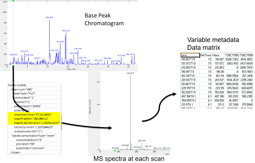 --- ## XCMS 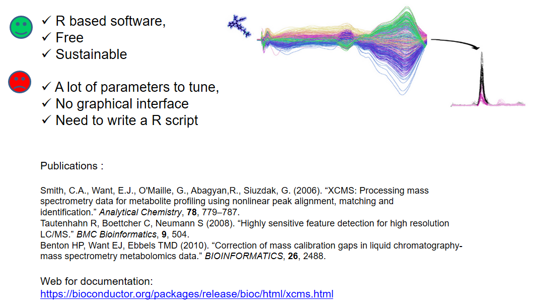 --- name:findchrompeaks ## xcms - findChromPeaks 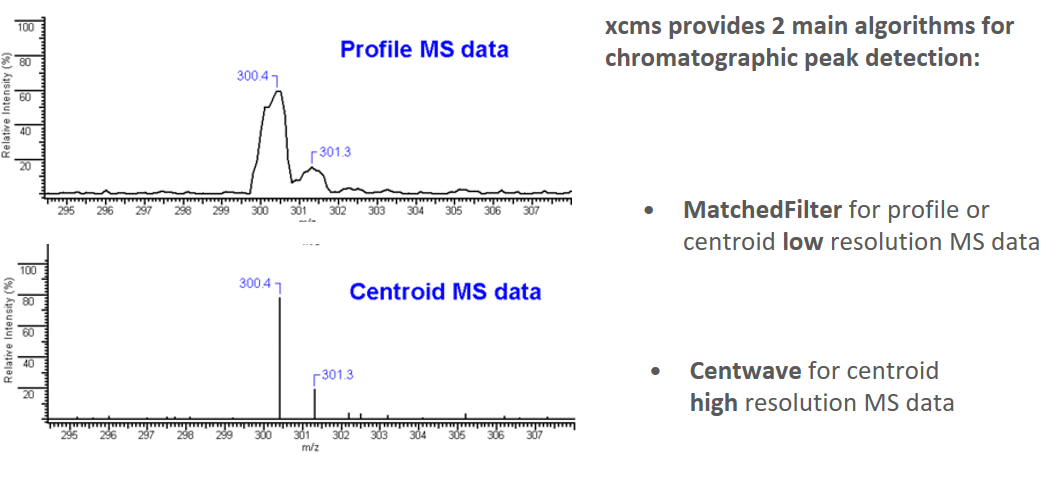 --- ## xcms - findChromPeaks - CentWave algorithm 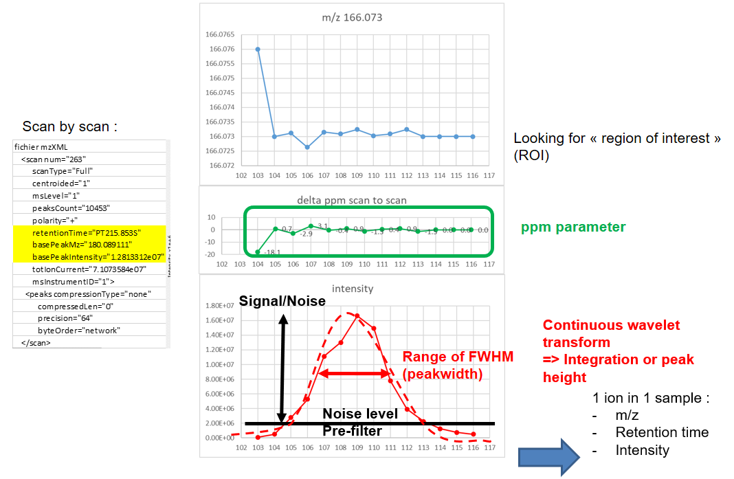 --- ## xcms - findChromPeaks - CentWave algorithm  --- ## xcms - findChromPeaks - CentWave algorithm  --- ## xcms - findChromPeaks - CentWave algorithm  --- ## xcms - findChromPeaks - CentWave parameters  --- ## xcms - findChromPeaks - Parameters summary xcms parameters | related to | description | examples --- | --- | --- | --- ppm | m/z | fluctuation of m/z value (ppm) from scan to scan - depends on the mass spectrometer accuracy | 5… peakwidth | retention time | range of chromatographic peak width (second) | UPLC 10,40 / HPLC 20,120 mzdiff | m/z and retention time | minimum difference of m/z for peaks with overlapping retention time (coeluting peak) - must be negative to allow overlap | -0.001 or 0.05 prefilter (k, I) | Intensity | a peak must be present in k scans with an intensity greater than I | k=3,I=1000 snthresh | Intensity | signal/noise ratio threshold | 5… noise | Intensity | each centroid must be greater than the "noise" value | . --- name:groupchrompeaks ## xcms - groupChromPeaks 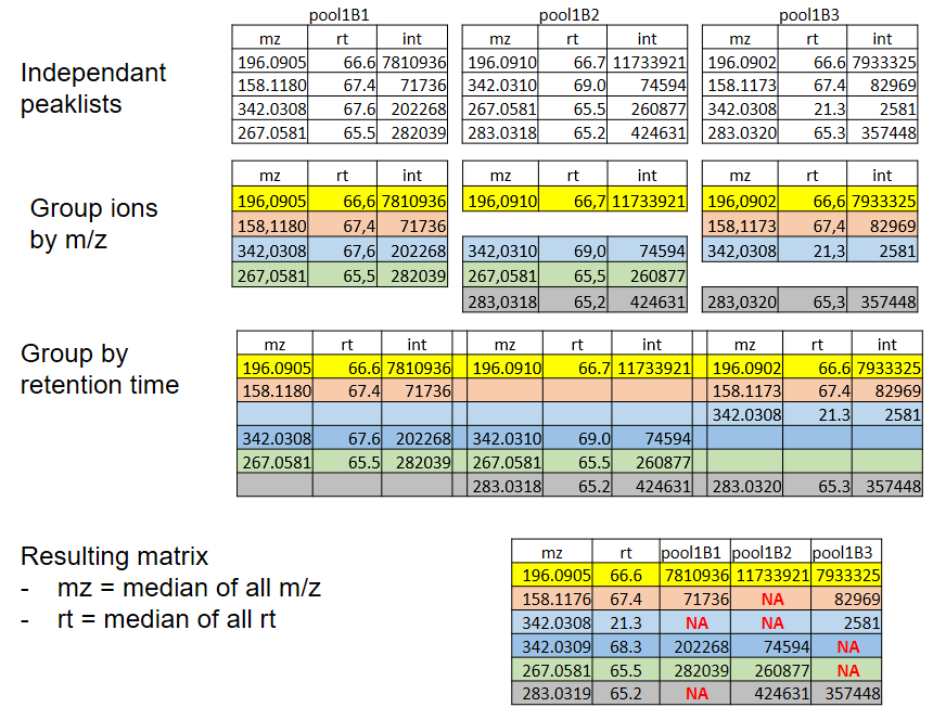 --- ## xcms - groupChromPeaks - Alignment group 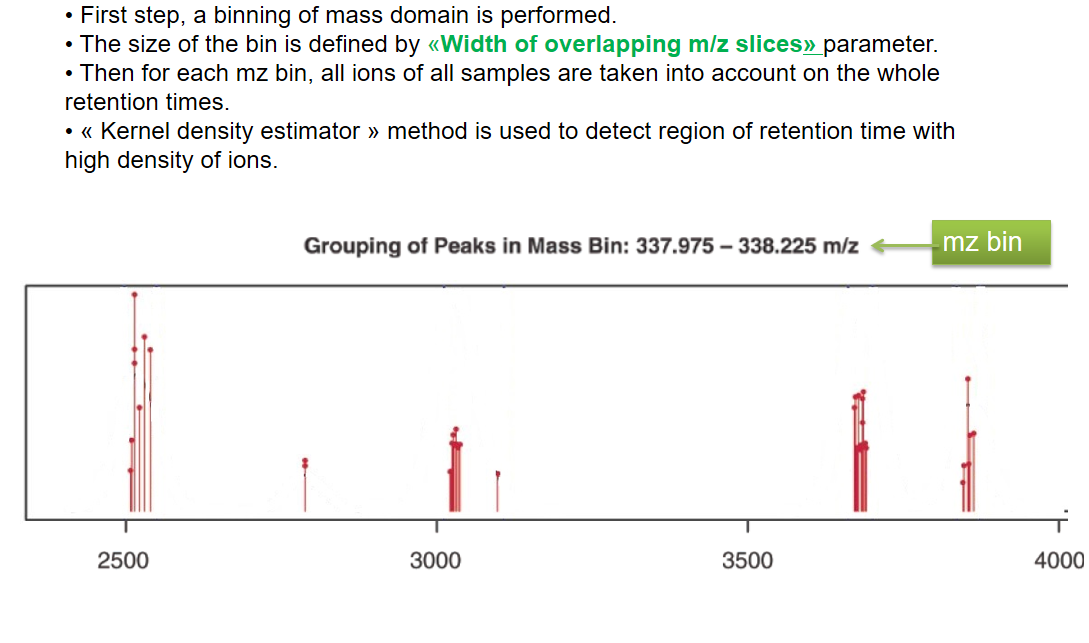 --- ## xcms - groupChromPeaks - Alignment group 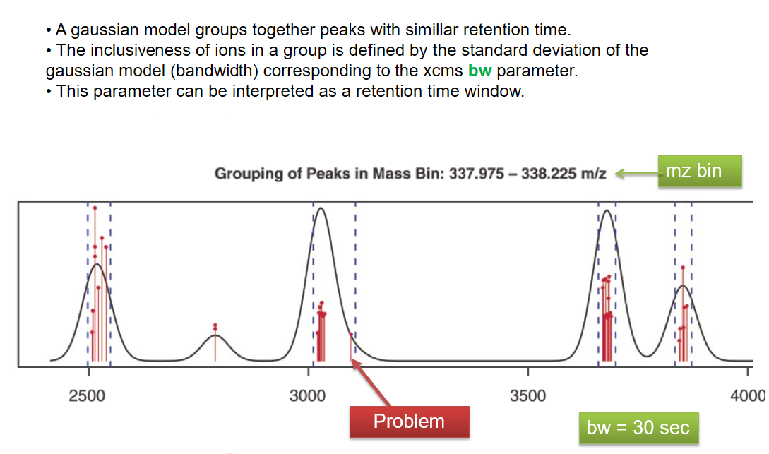 --- ## xcms - groupChromPeaks - Alignment group 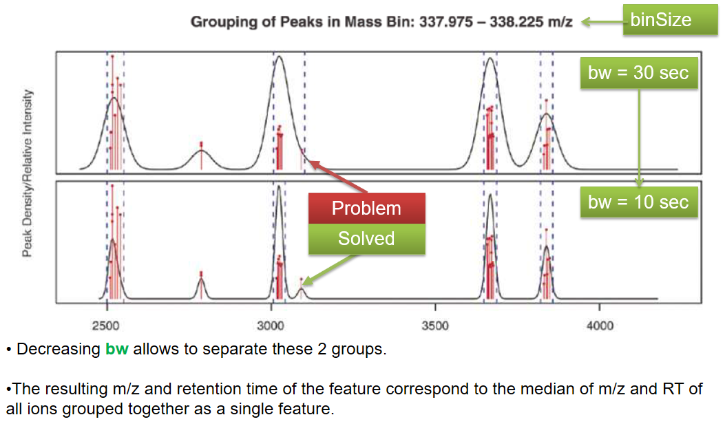 --- ## xcms - groupChromPeaks - minFraction parameter  --- ## xcms - groupChromPeaks - Output  --- ## xcms - groupChromPeaks - Output  --- ## xcms - groupChromPeaks - Parameters summary xcms parameters | related to | description | examples --- | --- | --- | --- binSize | m/z | Size of m/z slices (bins). Range of m/z to be included in a group. Depends on mass spectrometer accuracy. | bw | retention time | Standart deviation of the gaussian metapeak that group peaks together. | HPLC 30s / UPLC 5s minFraction | samples | To be valid, a group must be found in at least minFraction*n samples, with n=number of samples **for each class of samples**. A minFraction=0.5 corresponds to 50%. | n=10, minFraction=0.5 => found in at least 5 samples max | number of ions | Maximum number of groups detected in a single m/z slices. | 10 or 50 --- name:adjustrtime ## xcms - adjustRtime  --- ## xcms - adjustRtime - PeakGroups algorithm  --- ## xcms - adjustRtime - PeakGroups - Parameters summary xcms parameters | related to | description | examples --- | --- | --- | --- smooth method | retention time | Regression model to model time deviation among samples (linear or loess). | linear or loess span | | Degree of smoothing of the loess model. | 0.2 to 1 extraPeaks | samples | Number of "extra" peaks used to define reference peaks (or well-behaved peaks) for modeling time deviation. Number of Peaks > number of samples. | default=1 minFraction (previously missing) | samples | Minimum proportion of samples with reference peaks. If blank samples are used, minFraction < (1 - proportion of blanks). | 1 - proportion of blank samples --- ## xcms - adjustRtime - Obiwrap algorithm  --- name:beforeafterrt ## xcms - adjustRtime - Output  --- name:fillchrompeaks ## xcms - fillChromPeaks  --- --- ## Thank You! This material is the result of a collaborative work. Thanks to the [Galaxy Training Network](https://training.galaxyproject.org) and all the contributors! <div markdown="0"> <div class="contributors-line"> <table class="contributions"> <tr> <td><abbr title="These people wrote the bulk of the tutorial, they may have done the analysis, built the workflow, and wrote the text themselves.">Author(s)</abbr></td> <td> <a href="/training-material/hall-of-fame/jfrancoismartin/" class="contributor-badge contributor-jfrancoismartin"><img src="https://avatars.githubusercontent.com/jfrancoismartin?s=36" alt="Jean-François Martin avatar" width="36" class="avatar" /> Jean-François Martin</a><a href="/training-material/hall-of-fame/melpetera/" class="contributor-badge contributor-melpetera"><img src="https://avatars.githubusercontent.com/melpetera?s=36" alt="Mélanie Petera avatar" width="36" class="avatar" /> Mélanie Petera</a> </td> </tr> <tr class="reviewers"> <td><abbr title="These people reviewed this material for accuracy and correctness">Reviewers</abbr></td> <td> <a href="/training-material/hall-of-fame/shiltemann/" class="contributor-badge contributor-badge-small contributor-shiltemann"><img src="https://avatars.githubusercontent.com/shiltemann?s=36" alt="Saskia Hiltemann avatar" width="36" class="avatar" /></a><a href="/training-material/hall-of-fame/lecorguille/" class="contributor-badge contributor-badge-small contributor-lecorguille"><img src="https://avatars.githubusercontent.com/lecorguille?s=36" alt="Gildas Le Corguillé avatar" width="36" class="avatar" /></a><a href="/training-material/hall-of-fame/foellmelanie/" class="contributor-badge contributor-badge-small contributor-foellmelanie"><img src="https://avatars.githubusercontent.com/foellmelanie?s=36" alt="Melanie Föll avatar" width="36" class="avatar" /></a><a href="/training-material/hall-of-fame/melpetera/" class="contributor-badge contributor-badge-small contributor-melpetera"><img src="https://avatars.githubusercontent.com/melpetera?s=36" alt="Mélanie Petera avatar" width="36" class="avatar" /></a><a href="/training-material/hall-of-fame/bgruening/" class="contributor-badge contributor-badge-small contributor-bgruening"><img src="https://avatars.githubusercontent.com/bgruening?s=36" alt="Björn Grüning avatar" width="36" class="avatar" /></a><a href="/training-material/hall-of-fame/gallardoalba/" class="contributor-badge contributor-badge-small contributor-gallardoalba"><img src="https://avatars.githubusercontent.com/gallardoalba?s=36" alt="Cristóbal Gallardo avatar" width="36" class="avatar" /></a></td> </tr> </table> </div> </div> <div style="display: flex;flex-direction: row;align-items: center;justify-content: center;"> <img src="/training-material/assets/images/GTNLogo1000.png" alt="Galaxy Training Network" style="height: 100px;"/> </div> Tutorial Content is licensed under <a rel="license" href="http://creativecommons.org/licenses/by/4.0/">Creative Commons Attribution 4.0 International License</a>.<br/>