Frequently Asked Questions
Tutorial Questions
ANI threshold for dereplication
Selecting an appropriate ANI threshold for de-replication depends on the specific goals of your analysis. ANI measures the similarity between genomes, but the threshold for considering genomes “the same” varies by application. Two key parameters influence this decision:
- Minimum secondary ANI: The lowest ANI value at which genomes are considered identical.
- Minimum aligned fraction: The minimum genome overlap required to trust the ANI calculation.
These parameters are determined by the secondary clustering algorithm used in tools like dRep ( Galaxy version 3.6.2+galaxy1)
Common Use Cases and Thresholds
Species-Level De-Replication
For generating Species-Level Representative Genomes (SRGs), a 95% ANI threshold is widely accepted. This threshold was used in studies like Almeida et al. 2019 to create a comprehensive set of high-quality reference genomes for human gut microbes. While there is debate about whether bacterial species exist as discrete units or a continuum, 95% ANI remains a practical standard for species-level comparisons. For context, see Olm et al. 2017.
Avoiding Read Mis-Mapping
If the goal is to prevent mis-mapping of short metagenomic reads (typically (( \sim )) 150 bp), a stricter 98% ANI threshold is recommended. At this level, reads are less likely to map equally well to multiple genomes, ensuring clearer distinctions between closely related strains.
Default and Practical Considerations
- Default ANI threshold in dRep: 95% (suitable for most species-level applications).
- Upper limit for detection: Thresholds up to 99.9% are generally reliable, but higher values (e.g., 100%) are impractical due to algorithmic limitations (e.g., genomic repeats). Self-comparisons typically yield (( \sim )) 99.99% ANI due to these constraints.
- For strain-level comparisons, consider using InStrain ( Galaxy version 1.5.3+galaxy0) (Olm et al. 2021), which provides detailed strain-resolution analyses.
Important Notes
- De-replication collapses closely related but non-identical strains/genomes. This is inherent to the process.
- To explore strain-level diversity after de-replication, map original reads back to the dereplicated genomes and visualize the strain cloud using tools like InStrain (Bendall et al. 2016).
For further discussion on ANI thresholds, see Are these microbes the “same”? (Blog Post)
Average Nucleotide Identity (ANI): A Measure of Genomic Similarity
Average Nucleotide Identity (ANI) is a computational metric used to quantify the genomic similarity between two microbial genomes. It measures the mean sequence identity across all orthologous regions—regions of the genome that are shared and aligned between the two organisms. ANI is widely used in microbial genomics and metagenomics to:
- Compare the similarity of bacterial or archaeal genomes.
- Define species boundaries (e.g., a threshold of 95–96% ANI is commonly used to delineate bacterial species).
- Identify redundant genomes in datasets, such as Metagenome-Assembled Genomes (MAGs), for de-replication.
How ANI Is Calculated
- Genome Alignment: The genomes of two organisms are compared using whole-genome alignment tools (e.g., BLAST, MUMmer, or FastANI). These tools identify regions of the genomes that are homologous (shared due to common ancestry).
- Identity Calculation: For each aligned region, the percentage of identical nucleotides is calculated. ANI is then computed as the mean identity across all aligned regions that meet a specified length threshold (e.g., regions \( \geq \) 1,000 base pairs).
- Normalization: ANI accounts for unaligned regions (e.g., due to genomic rearrangements or horizontal gene transfer) by focusing only on the aligned portions of the genomes. This ensures the metric reflects conserved genomic similarity rather than absolute sequence coverage.
Interpreting ANI Values ANI values range from 0% to 100%, where:
- ANI \( \approx \) 100%: The genomes are nearly identical, likely representing strains of the same species or clones.
- ANI \( \geq \) 95–96%: The genomes likely belong to the same species (a widely accepted threshold for bacterial species delineation).
- ANI \( \approx \) 80–95%: The genomes belong to closely related species within the same genus.
- ANI \( < \) 80%: The genomes are distantly related and likely belong to different genera or higher taxonomic ranks.
Applications of ANI
- Species Delineation: ANI is a gold standard for defining microbial species, replacing or complementing traditional methods like DNA-DNA hybridization (DDH). For example, an ANI \(\geq \) 95% is often used to confirm that two genomes belong to the same species.
- De-Replication of MAGs: In metagenomics, ANI is used to identify and remove redundant MAGs from datasets. MAGs with ANI values above a threshold (e.g., 99%) are considered redundant, and only the highest-quality representative is retained for downstream analysis.
- Strain-Level Comparisons: ANI can distinguish between closely related strains of the same species, helping researchers study microbial diversity at fine taxonomic resolutions.
- Taxonomic Classification: ANI is used to assign unknown genomes to known taxonomic groups by comparing them to reference genomes in databases.
Tools for Calculating ANI
Several bioinformatics tools are available to compute ANI, including:
- FastANI ( Galaxy version 1.3) (Jain et al. 2018): A fast, alignment-free tool for estimating ANI between genomes.
- PyANI: A Python-based tool that supports multiple ANI calculation methods (e.g., BLAST, MUMmer).
Limitations of ANI
While ANI is a powerful metric, it has some limitations:
- Dependence on Alignment: ANI requires sufficiently aligned regions to be accurate. Highly divergent or rearranged genomes may yield unreliable ANI values.
- Threshold Variability: The ANI threshold for species delineation (e.g., 95%) may vary depending on the microbial group or study context.
- Computational Requirements: Calculating ANI for large datasets (e.g., thousands of MAGs) can be computationally intensive.
Average Nucleotide Identity (ANI) is a fundamental metric in microbial genomics, providing a robust way to compare genomes, define species, and refine metagenomic datasets. By leveraging ANI, researchers can ensure the accuracy and reliability of their genomic analyses, from species classification to de-replication of MAGs.
CheckM2 vs CheckM
CheckM2 (Chklovski et al. 2023) is the successor of CheckM, but CheckM is still widely used, since its marker-based logic can be more interpretable in a biological sense. E.g., to date (2025-11-21), NCBI still allows submitting MAGs to GenBank if either checkM or checkM2 has a completeness of > 90% (see the NCBI WGS/MAG submission guidelines).
Key differences compared to CheckM:
- CheckM relies primarily on lineage-specific single-copy marker genes to estimate completeness and contamination of microbial genomes.
- CheckM2 uses a machine-learning (gradient boost / ML) approach trained on simulated and experimental genomes, and does not strictly require a well-represented lineage in its marker database.
- CheckM2 is reported to be more accurate and faster for both bacterial and archaeal lineages, especially when dealing with novel or very reduced-genome lineages (e.g., candidate phyla, CPR/DPANN) where classical marker-gene methods may struggle.
- The database of CheckM2 can be updated more rapidly with new high-quality reference genomes, which supports scalability and improved performance over time.
If you’re working with MAGs from underrepresented taxa (novel lineages) or very small genomes (streamlined bacteria/archaea), CheckM2 tends to give more reliable estimates of completeness/contamination. For more “standard” microbial genomes from well-studied taxa, CheckM may still work well, but you may benefit from the improved performance with CheckM2.
Maximum MAG contamination percentage
Contamination in Metagenome-Assembled Genomes (MAGs) refers to the presence of sequences from organisms other than the target organism. During de-replication, setting a maximum contamination threshold ensures that only high-quality, representative genomes are retained for downstream analyses.
Why Set a Maximum Contamination Threshold?
Data Quality:
High contamination can distort taxonomic classification, functional annotation, and comparative genomics. A contamination threshold ensures that only high-purity MAGs are included.
Accurate De-Replication:
Contaminated MAGs may cluster incorrectly, leading to misrepresentation of microbial diversity. A contamination threshold helps ensure that only genuinely similar genomes are grouped together.
Functional and Ecological Insights: Low-contamination MAGs provide more reliable insights into microbial functions and ecological roles.
Default and Common Contamination Thresholds
The default contamination threshold in dRep is 25%, which balances inclusivity and quality for general metagenomic studies. However, the choice of threshold depends on the specific goals of your analysis:
Threshold Use Case < 5% Ideal for high-confidence analyses, such as reference genomes or species-level comparisons. < 10% Suitable for most metagenomic studies, balancing purity and genome diversity. < 25% Default in dRep, allowing for broader genome inclusion while maintaining reasonable purity.
< 5% Contamination: Used for high-quality MAGs intended for reference databases or detailed functional analyses.
< 10% Contamination: A widely adopted threshold for general metagenomic studies, balancing purity and genome retention.
< 25% Contamination: The default in dRep, this threshold is more permissive, allowing for a broader range of MAGs while still maintaining reasonable quality.
How to Choose the Right Threshold
Study Goals: For high-quality reference databases, use a < 5% threshold. For general analyses, < 10% is recommended. The default 25% in dRep is suitable for exploratory studies.
Tool Recommendations: Tools like dRep and CheckM provide contamination estimates and allow you to set thresholds based on your needs.
Trade-Offs: Stricter thresholds (e.g., < 5%) will exclude more MAGs, potentially reducing dataset diversity. More permissive thresholds (e.g., < 25%) will retain more MAGs but may include lower-quality genomes.
Setting a maximum contamination threshold is essential for ensuring the quality of de-replicated MAGs. The default threshold in dRep is 25%, but you can adjust it based on your study goals and the trade-offs between purity and genome retention. By carefully selecting this threshold, you can optimize your MAG dataset for accurate downstream analyses.
Minimum MAG completeness percentage
Choosing a minimum genome completeness threshold is a critical but complex decision in de-replication and bin refinement. There is a trade-off between computational efficiency and genome quality:
- Lower completeness thresholds allow more genomes to be included but reduce the accuracy of similarity comparisons.
- Higher completeness thresholds improve accuracy but may exclude valuable genomes.
Impact of Genome Completeness on Aligned Fractions
When genomes are incomplete, the aligned fraction—the proportion of the genome that can be compared—decreases. For example, if you randomly sample 20% of a genome twice, the aligned fraction between these subsets will be low, even if they originate from the same genome.
This effect is illustrated below, where lower completeness thresholds result in a wider range of aligned fractions, reducing the reliability of similarity metrics like ANI.
Effect on Mash ANI
Incomplete genomes also artificially lower Mash ANI values, even for identical genomes. As completeness decreases, the reported Mash ANI drops, even when comparing identical genomes.
This is problematic because Mash is used for primary clustering in tools like dRep. If identical genomes are split into different primary clusters due to low Mash ANI, they will never be compared by the secondary algorithm and thus won’t be de-replicated.
Practical Implications for De-Replication
Primary Clustering Thresholds:
If you set a minimum completeness of 50%, identical genomes subset to 50% may only achieve a Mash ANI of \( \approx \) 96%. To ensure these genomes are grouped in the same primary cluster, the primary clustering threshold must be \( \leq \) 96%. Otherwise, they may be incorrectly separated.
Computational Trade-Offs:
Lower primary thresholds increase the size of primary clusters, leading to more secondary comparisons and longer runtimes. Higher thresholds improve speed but risk missing true matches.
Unknown Completeness:
In practice, the true completeness of genomes is often unknown. Tools like CheckM estimate completeness using single-copy gene inventories, but these estimates are not perfect in particular for phages and plasmids, explaining why they are not supported in dRep. In general though, checkM is pretty good at accessing genome completeness:
Guidelines for Setting Completeness Thresholds
- Avoid thresholds below 50% completeness: Genomes below this threshold are often too fragmented for reliable comparisons, and secondary algorithms may fail.
- Adjust Mash ANI thresholds accordingly: If you lower the secondary ANI threshold, also lower the Mash ANI threshold to ensure incomplete but similar genomes are grouped together.
Balancing genome completeness and computational efficiency is key to effective de-replication. While lower completeness thresholds include more genomes, they reduce alignment accuracy and increase runtime. Aim for a minimum completeness of \( \geq \)50% and adjust clustering thresholds to avoid splitting identical genomes.

, Mash ANI is severely impacted. Source: <a href='https://drep.readthedocs.io/en/latest/choosing_parameters.html#importance-of-genome-completeness'>dRep documentation</a>")

Minimum MAG length
In dRep, the set of Metagenome-Assembled Genomes (MAGs) undergoes quality filtering before any comparisons are performed. This critical step ensures that only high-quality genomes are retained for downstream analysis, improving both accuracy and computational efficiency.
One of the first steps in quality filtering is length-based filtering. Genomes that do not meet the minimum length threshold are filtered out upfront. This avoids unnecessary CheckM computations and ensures that only sufficiently large genomes are processed.
Important Note: All genomes must contain at least one predicted Open Reading Frame (ORF). Without an ORF, CheckM may stall during processing. To prevent this, a minimum genome length of 10,000 base pairs (bp) is recommended.
The default minimum length threshold in dRep is 50,000 bp. This threshold strikes a balance between computational efficiency and genome quality, ensuring that only meaningful and sufficiently complete genomes are included in the de-replication process.
Format
Kraken2 and the k-mer approach for taxonomy classification
In the \(k\)-mer approach for taxonomy classification, we use a database containing DNA sequences of genomes whose taxonomy we already know. On a computer, the genome sequences are broken into short pieces of length \(k\) (called \(k\)-mers), usually 30bp.
Kraken examines the \(k\)-mers within the query sequence, searches for them in the database, looks for where these are placed within the taxonomy tree inside the database, makes the classification with the most probable position, then maps \(k\)-mers to the lowest common ancestor (LCA) of all genomes known to contain the given \(k\)-mer.
Kraken2 uses a compact hash table, a probabilistic data structure that allows for faster queries and lower memory requirements. It applies a spaced seed mask of s spaces to the minimizer and calculates a compact hash code, which is then used as a search query in its compact hash table; the lowest common ancestor (LCA) taxon associated with the compact hash code is then assigned to the k-mer.
You can find more information about the Kraken2 algorithm in the paper Improved metagenomic analysis with Kraken 2.
 of the genomes that contain that k-mer in the database. The taxa associated with the sequence's k-mers, as well as the taxa's ancestors, form a pruned subtree of the general taxonomy tree, which is used for classification. In the classification tree, each node has a weight equal to the number of k-mers in the sequence associated with the node's taxon. Each root-to-leaf (RTL) path in the classification tree is scored by adding all weights in the path, and the maximal RTL path in the classification tree is the classification path (nodes highlighted in yellow). The leaf of this classification path (the orange, leftmost leaf in the classification tree) is the classification used for the query sequence. Source: <span class=\"citation\"><a href=\"#Wood2014\">Wood and Salzberg 2014</a></span>")
What is Taxonomy?
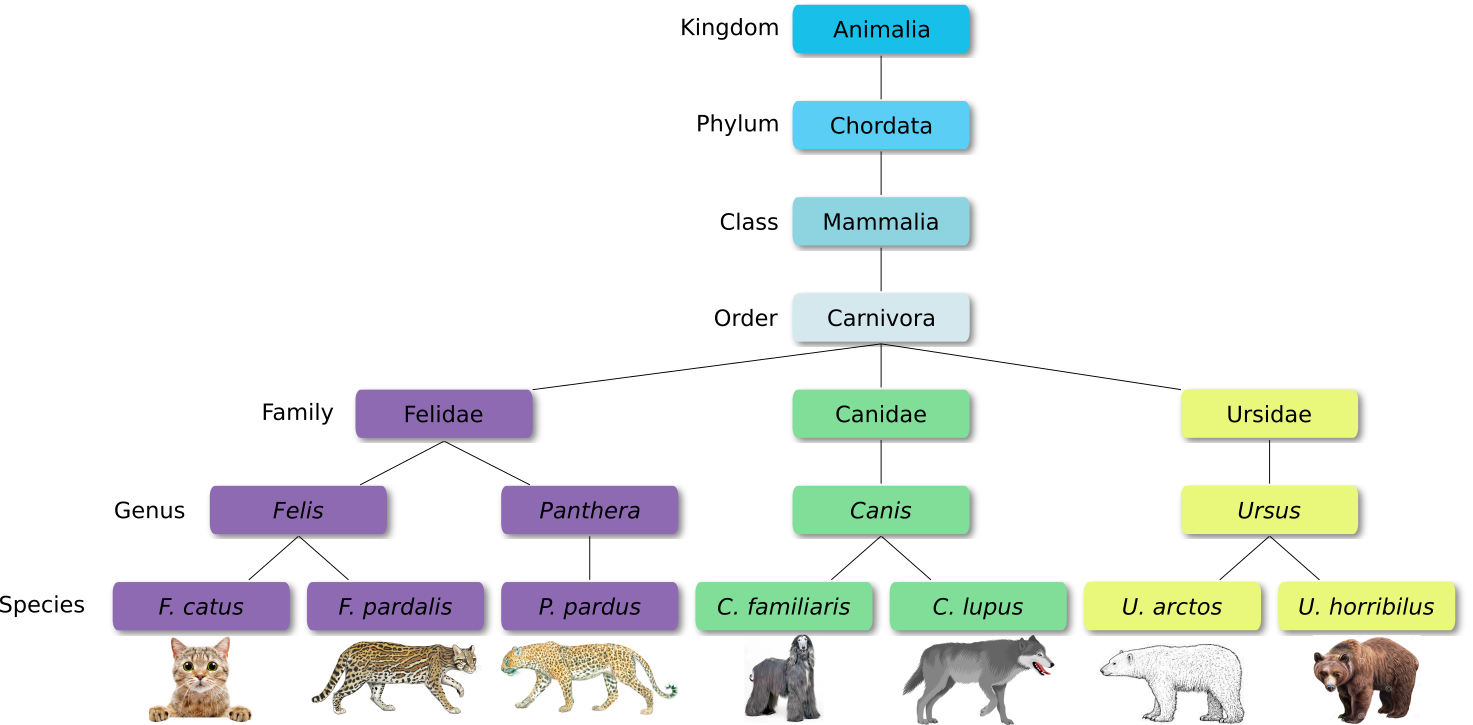
Taxonomy is the method used to naming, defining (circumscribing) and classifying groups of biological organisms based on shared characteristics such as morphological characteristics, phylogenetic characteristics, DNA data, etc. It is founded on the concept that the similarities descend from a common evolutionary ancestor.
Defined groups of organisms are known as taxa. Taxa are given a taxonomic rank and are aggregated into super groups of higher rank to create a taxonomic hierarchy. The taxonomic hierarchy includes eight levels: Domain, Kingdom, Phylum, Class, Order, Family, Genus and Species.
The classification system begins with 3 domains that encompass all living and extinct forms of life
- The Bacteria and Archae are mostly microscopic, but quite widespread.
- Domain Eukarya contains more complex organisms
When new species are found, they are assigned into taxa in the taxonomic hierarchy. For example for the cat:
Level Classification Domain Eukaryota Kingdom Animalia Phylum Chordata Class Mammalia Order Carnivora Family Felidae Genus Felis Species F. catus From this classification, one can generate a tree of life, also known as a phylogenetic tree. It is a rooted tree that describes the relationship of all life on earth. At the root sits the “last universal common ancestor” and the three main branches (in taxonomy also called domains) are bacteria, archaea and eukaryotes. Most important for this is the idea that all life on earth is derived from a common ancestor and therefore when comparing two species, you will -sooner or later- find a common ancestor for all of them.
Let’s explore taxonomy in the Tree of Life, using Lifemap
References
- Wood, D. E., and S. L. Salzberg, 2014 Kraken: ultrafast metagenomic sequence classification using exact alignments. Genome Biology 15: R46. 10.1186/gb-2014-15-3-r46
- Olm, M. R., C. T. Brown, B. Brooks, and J. F. Banfield, 2017 dRep: a tool for fast and accurate genomic comparisons that enables improved genome recovery from metagenomes through de-replication. The ISME journal 11: 2864–2868. 10.1038/ismej.2017.126
- Jain, C., L. M. Rodriguez-R, A. M. Phillippy, K. T. Konstantinidis, and S. Aluru, 2018 High throughput ANI analysis of 90K prokaryotic genomes reveals clear species boundaries. Nature Communications 9: 10.1038/s41467-018-07641-9
- Almeida, A., A. L. Mitchell, M. Boland, S. C. Forster, G. B. Gloor et al., 2019 A new genomic blueprint of the human gut microbiota. Nature 568: 499–504. 10.1038/s41586-019-0965-1
- Olm, M. R., A. Crits-Christoph, K. Bouma-Gregson, B. A. Firek, M. J. Morowitz et al., 2021 inStrain profiles population microdiversity from metagenomic data and sensitively detects shared microbial strains. Nature Biotechnology 39: 727–736. 10.1038/s41587-020-00797-0
- Chklovski, A., D. H. Parks, B. J. Woodcroft, and G. W. Tyson, 2023 CheckM2: a rapid, scalable and accurate tool for assessing microbial genome quality using machine learning. Nature methods 20: 1203–1212. 10.1101/2022.07.11.499243