You may already know that there are different types of -omic sciences; out of these, metabolomics is most closely related to phenotypes. Metabolomics involves the study of different types of matrices, such as blood, urine, tissues, in various organisms including plants. It focuses on studying the very small molecules which are called metabolites, to better understand matters linked to the metabolism. However, studying metabolites is not a piece of cake since it requires several critical steps which still have some major bottlenecks. Metabolomics is still quite a young science, and has many kinds of specific challenges.
One of the three main technologies used to perform metabolomic analysis is Gas-Chromatography Mass Spectrometry (GC-MS). Data analysis for this technology requires a large variety of steps, ranging from extracting information from the raw data, to statistical analysis and annotation. Many packages in R/Python are available for the analysis of GC-MS or LC-MS (Liquid-Chromatography Mass Spectrometry) data - for more details see the reviews by Stanstrup et al. 2019 and Misra 2021.
This tutorial explains the main steps involved in untargeted GC-MS data processing. To do so we focus on some open-source solutions integrated within the Galaxy framework, namely XCMS and metaMS. The selected tools and functionalities only covers a small portion of available tools but allow to perform a complete GC-MS analysis in a single environment.
In this tutorial, we will learn how to (1) extract features from the raw data using XCMS (Smith et al. 2006), (2) deconvolute the detected features into spectra with metaMS (Wehrens et al. 2014) and (3) annotate unknow spectra using spectral database comparison tools.
To illustrate this approach, we will use data from Dittami et al. 2012. Due to time constraints in processing the original dataset, a limited subset of samples was used to illustrate the workflow. This subset (see details below) demonstrates the key steps of metabolomics analysis, from pre-processing to annotation. Although the results derived from this reduced sample size may not be scientifically robust, they provide insight into essential methodological foundations of GC-MS data-processing workflow.
The objective of the study conducted by Dittami et al. was to investigate the adaptation mechanisms of the brown algae Ectocarpus to low-salinity environments. The research focused on examining physiological tolerance and metabolic changes in freshwater and marine strains of Ectocarpus. Using transcriptomic (gene expression profiling) and metabolic analyses, the authors identified significant, reversible changes occurring in the freshwater strain when exposed to seawater. Both strains exhibited similarities in gene expression under identical conditions; however, substantial differences were observed in metabolite profiles.
The study utilized a freshwater strain of Ectocarpus and a marine strain for comparative analysis. The algae were cultured in media with varying salinities, prepared by diluting natural seawater or adding NaCl. The algae were acclimated to these conditions before extraction.
The six samples used in this training were analyzed by GC-MS (low resolution instrument). A marine strain raised in sea water media (2 replicates) and freshwater strains raised in either 5% or 100% sea water media (2 replicates each). The training dataset is available on Zenodo
To process the GC-MS data, we can use several tools. One of these is XCMS (Smith et al. 2006), a general R package for untargeted metabolomics profiling. It can be used for any type of mass spectrometry acquisition (centroid and profile) and resolution (from low to high resolution), including FT-MS data coupled with a different kind of chromatography (liquid or gas). Because of the generality of packages like XCMS, several other packages have been developed to use the functionalities of XCMS for optimal performance in a particular context. The R package called metaMS (Wehrens et al. 2014) does so for the field of GC-MS untargeted metabolomics. One of the goals of metaMS was to set up a simple system with few user-settable parameters, capable of handling untargeted metabolomics experiments.
In this tutorial we use XCMS to detect chromatographic peaks within our samples. Once we have detected them, they need to be deconvoluted into mass spectra representing chemical compounds. For that, we use metaMS functions. To normalize the retention time of deconvoluted spectra in our sample, we compute the retention index using Alkane references and a dedicated function of metaMS. Finally, we identify detected spectra by aligning them with a database of known compounds. This can be achieved using an in-house built database in the common MSP format (.msp) (used in the NIST MS search program for example), resulting in a table of annotated compounds.
Comment
In Galaxy other GC-MS data processing workflows are available and may be of interest for more advanced Galaxy users (see the Metabolomics section).
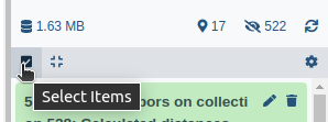
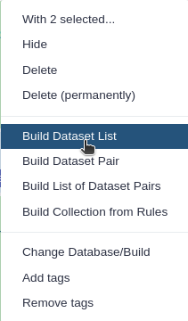
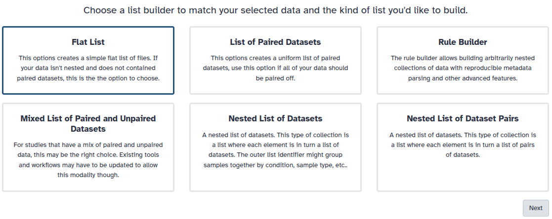
Before we can start with the actual analysis pipeline, we first need to download and prepare our dataset. Many of the preprocessing steps can be run in parallel on individual samples. Therefore, we recommend using the Dataset collections in Galaxy. This can be achieved by using the dataset collection option from the beginning of your analysis when uploading your data into Galaxy.
Import the data into Galaxy
Hands On: Upload data
Create a new history for this tutorial
To create a new history simply click the new-history icon at the top of the history panel:
Click galaxy-uploadUpload at the top of the activity panel
Select galaxy-wf-editPaste/Fetch Data
Paste the link(s) into the text field
Press Start
Close the window
Comment: The extra files
The three additional files contain the reference_alkanes, the W4M0004_database_small, and the sampleMetadata. Those files are auxiliary inputs used in the data processing and contain either extra information about the samples or serve as reference data for indexing and identification.
The reference_alkanes (.tsv or .csv) with retention times and carbon number or retention index is used to compute the retention index of the deconvoluted peaks. The alkanes should be measured in the same batch as the input sample collection.
The W4M0004_database_small (.msp) is a reference database used for the identification of spectra. It contains the recorded and annotated mass spectra of chemical standards, ideally from a similar instrument. The unknown spectra which can be detected in the sample can then be confirmed via comparison with this library. The specific library is an in-house library of metabolite standards extracted with metaMS .
The sample metadata (.csv or .tsv) is a table containing information about our samples. In particular, the tabular file contains for each sample its associated sample name, class (SW, FWS, etc.). It is possible to add more columns to include additional details about the samples (e.g : batch number, injection order…).
As a result of this step, you should have in our history a green Dataset collection param-collection with all 6 samples .mzML files as well as three separate files with reference alkanes, reference spectral library, and sample metadata.
Create the XCMS object
The first part of data processing is using the XCMS tool to detect peaks in the MS signal. For that, we first need to take the .mzML files and create a format usable by the XCMS tool. MSnbase readMSData ( Galaxy version 2.16.1+galaxy0) (Gatto and Lilley 2012. Gatto et al. 2020) takes as input our files and prepares RData files for the first XCMS step.
Comment
The MSnbase readMSDatatool function, prior to XCMS, is able to read files with open format as mzXML, mzML, mzData and netCDF, which are independent of the manufacturers’ proprietary formats. Working with open MS data file format allows users to us tools developed outside of the MS instrument provider. This set of packages/functions gives modularity, and thus is particularly well adapted to define workflows, one of the key points of Galaxy.
Hands On: Create the XCMS object
MSnbase readMSData ( Galaxy version 2.16.1+galaxy0) with the following parameters:
param-collection“File(s) from your history containing your chromatograms”: input
Click on param-collectionDataset collection in front of the input parameter you want to supply the collection to.
Select the collection you want to use from the list
The output should be input.raw.RData
This dataset is a collection of rdata.msnbase.raw files. That Rdata file is necessary in the next step of the workflow. It contains an internal R representation of XCMS objects.
As a result of this step, you should have in your history a new green dataset collection called input.raw.RData that will serve as input for the next processing step: peak picking.
Peak detection using XCMS
The first step in the workflow is to detect the peaks in our data using XCMS functions. This part, however, is covered by a separate tutorial. Although the tutorial is dedicated to LC-MS data, it can also be followed for our GC-MS data. Therefore, in this section, we do not explain this part of the workflow in detail but rather refer the reader to the dedicated tutorial. Please also pay attention to the parameter values for individual Galaxy tools, as these can differ from the referred tutorial and are adjusted to our GC-MS dataset.
Since this step is already covered in a separate tutorial, it is possible to skip it. Instead, you can go directly to Peak deconvolution step using a preprocessed XCMS object file prepared for you.
Click galaxy-uploadUpload at the top of the activity panel
Select galaxy-wf-editPaste/Fetch Data
Paste the link(s) into the text field
Press Start
Close the window
The format of uploaded file containing XCMS object should be .RData.
Allow Galaxy to detect the datatype during Upload, and adjust from there if needed.
Tool forms will filter for the appropriate datatypes it can use for each input.
Directly changing a datatype can lead to errors. Be intentional and consider converting instead when possible.
Dataset content can also be adjusted (tools: Data manipulation) and the expected datatype detected. Detected datatypes are the most reliable in most cases.
If a tool does not accept a dataset as valid input, it is not in the correct format with the correct datatype.
Once a dataset’s content matches the datatype, and that dataset is repeatedly used (example: Reference annotation) use that same dataset for all steps in an analysis or expect problems. This may mean rerunning prior tools if you need to make a correction.
Tip: Not sure what datatypes a tool is expecting for an input?
Create a new empty history
Click on a tool from the tool panel
The tool form will list the accepted datatypes per input
Warning: In some cases, tools will transform a dataset to a new datatype at runtime for you.
This is generally helpful, and best reserved for smaller datasets.
Why? This can also unexpectedly create hidden datasets that are near duplicates of your original data, only in a different format.
For large data, that can quickly consume working space (quota).
Deleting/purging any hidden datasets can lead to errors if you are still using the original datasets as an input.
Consider converting to the expected datatype yourself when data is large.
Then test the tool directly on converted data. If it works, purge the original to recover space.
The first step (called peak picking) is to extract peaks from each of your data files independently. For this purpose, we use the MatchedFilter chromatographic peak detection algorithm implemented in xcms findChromPeaks (xcmsSet) ( Galaxy version 3.12.0+galaxy0).
One Galaxy Training material already explains how to act with MS data. We encourage you to follow this link and complete the corresponding tutorial: Mass spectrometry: LC-MS preprocessing with XCMS.
For GC-MS analysis you don’t really need to follow all of this previous tutorial but for a better understanding of your data, it is recommended to try it with their test dataset.
Concerning the current GC-MS tutorial, you just have to compute the following steps and specific parameters described in the hands-on part below (please follow the parameter values below to obtain the same results during the training).
Hands On: Peak picking of GC-MS data with XCMS
xcms findChromPeaks (xcmsSet) ( Galaxy version 3.12.0+galaxy0) with the following parameters:
param-collection“RData file”: input.raw.RData (the output collection of files from the MSnbase readMSDatatool step)
“Extraction method for peaks detection”: MatchedFilter - peak detection in chromatographic space
“Full width at half maximum of matched filtration gaussian model peak”: 5
“Step size to use for profile generation”: 0.5
In “Advanced Options”:
“Maximum number of peaks that are expected/will be identified per slice”: 500
“Signal to Noise ratio cutoff”: 2
“Minimum difference in m/z for peaks with overlapping Retention Times”: 0.5
Comment
For GC-MS data in profile mode, use the MatchedFilter algorithm instead of the CentWave algorithm used in the LC-MS tutorial.
For low-resolution GC-MS data, a larger m/z difference (0.5 Da) can be used to separate overlapping peaks. If you have high-resolution data (from GC-ToF or GC-Orbitrap), you can use a smaller m/z difference (0.01 Da).
xcms findChromPeaks Merger ( Galaxy version 3.12.0+galaxy0) with the following parameters:
param-collection“RData file”: input.raw.xset.RData (output collection of files from the xcms findChromPeaks (xcmsSet)tool job)
param-file“Sample metadata file “: sampleMetadata.tsv (One of the uploaded files from Zenodo)
Comment
To merge your data, you need to input a sampleMetadata file containing filenames and their metadata informations like their class for example.
If you don’t add a sampleMetadata file, the xcms findChromPeaks Mergertool tool will group all your files together.
You can also create your sampleMetadata file with W4M Galaxy tool xcms get a sampleMetadata file ( Galaxy version 3.12.0+galaxy3) with the following parameters: param-collection“RData file”: input.raw.RData output from MSnbase readMSDatatool.
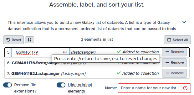
Here is an example of the minimum expectations about a sampleMetadata file (important: remove file extension from the sample names, file1.mzML should be file1):
sample_name
class
file1
marine strain
file2
pool
file3
freshwater strain
The output from xcms findChromPeaks Mergertool is an .RData file required for the next steps of the process.
There are two available options:
using the metaMS strategy specifically designed for GC-MS data deconvolution and annotation
using a full XCMS process for GC-MS data processing
Although this training material is dedicated to GC-MS analysis with the metaMS package, the two options are illustrated in this tutorial. Indeed, as mentioned in the introduction, metaMS is based on XCMS functions, with a specific adaptation to GC-MS data. Thus, one can be interested in comparing results that would be obtained with a standard XCMS processing. Consequently, the two options on the same dataset are available here.
Hands-on: Choose Your Own Tutorial
This is a 'Choose Your Own Tutorial' (CYOT) section (also known as 'Choose Your Own Analysis' (CYOA)), where you can select between multiple paths. Click one of the buttons below to select how you want to follow the tutorial
Choose below if you just want to follow the pipeline using metaMS or XCMS for GC-MS deconvolution and annotation
Processing with metaMS (option 1)
metaMS is an R package for MS-based metabolomics data. It was made to ease GC-MS data deconvolution and alignment steps using functions from XCMS and CAMERA packages. In its Galaxy implementation, the two main outputs of metaMS are: (1) a table of feature intensities in all samples, which can be analyzed with multivariate methods immediately, and (2) an MSP (.msp) file containing GC-MS spectra in a common spectral database format.
The biggest difference between XCMS only workflow (option 2) or XCMS + metaMS GC-MS data processing (option 1) is that rather than a feature-based analysis with individual peaks, as in the option 2 case, metaMS performs a pseudospectrum-based analysis and use it to align compound between samples. One other advantage is that metaMS allows creation of MSP (.msp) spectra export files ready for annotation.
Comment
Not all metaMS R package functions have been made available in Galaxy.
When run in R, the metaMS package offers a lot of possibilities. For more information on the full set of metaMS functions, visit the metaMS Bioconductor page.
During this part of the tutorial we are interested in GC-MS analysis with metaMS, so we will use the runGC function of metaMS and describe it in detail to understand all the capabilities of that function.
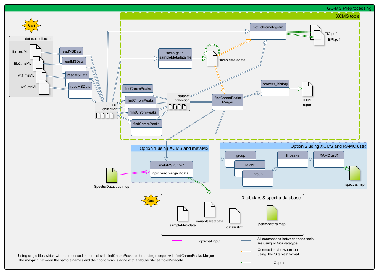
The standard workflow of metaMS for GC-MS data is the following:
The runGC function is implemented in metaMS.runGC tool tool in Galaxy. It takes as inputs an param-collection.RData file after XCMS peak picking and optionally for annotation purposes an alkane reference file (in either .csv or .tsv format) for RI calculation and/or a spectral database in .msp format.
Deconvolution and Alignment with metaMS
The peak picking is performed by the usual XCMS functions and the output file in .RData is used for deconvolution and Alignment steps with runGC function.
Hands On: metaMS.runGC
1.metaMS.runGC ( Galaxy version 3.0.0+metaMS1.24.0-galaxy0) with the following parameters:
param-file“Rdata from xcms and merged”: xset.merged.RData (output of the xcms findChromPeaks Mergertool step)
“Settings”: user_defined
“RT range option”: hide (If set to show you can limit the range of RT processed, for example remove solvant delays)
“RT_Diff”: 0.05 (Max time deviation in minute to cluster unknown pseudo-spectra between samples)
“Min_Features: 5 (Minimal number of features required to have a valid pseudo-spectrum, compound with less ions will be discarded)
“similarity_threshold”: 0.7 (Minimum cosine similarity between pseudo-spectra to be considers as equal)
“min.class.fract”: 0.5 (Minimal fraction of samples in which a pseudo-spectrum should be present to be kept)
“min.class.size”: 2 (Minimum number of samples in which a pseudo-spectrum should be find)
“Use Personnal DataBase option”: show (This activates the “DB file” selector)
param-file“DB file”: W4M0004_database_small.msp (The file download from Zenodo; if not available set the “Use Personnal DataBase option” to hide)
“Use RI option: show (Choose hide if you want to skip RI calculation)
param-file“RI file”: reference_alkanes.csv (Format should be strictly respected)
“Use RI as filter”: FALSE (If set to TRUE only unknown spectra with close RI as those in database will be kept)
“RIshift”: “not used”
Comment
For faster processing keep annotation modules off by setting “Use Personnal DataBase option”: hide and “Use RI option: hide
You can dataset-save download the MSP file and open it in your favorite spectra processing software or online database for further investigation!
The biggest difference between XCMS only or XCMS + metaMS GC-MS data processing is that rather than a feature-based analysis with individual peaks, as it is the case with XCMS, metaMS performs a pseudospectrum-based analysis. So, the basic entity is a set of m/z values showing a chromatographic peak at the same retention time. The idea behind that is that Electron Ionization (EI), which is the most widely used ionization mode in GC-MS analysis, generates a lot more ions for the same molecule than Electrospray Ionisation used in LC-MS. The runGC function from metaMS is able to group all ions belonging to a molecule into one single cluster that will be used for statistical analysis. For each compound found by metaMS, a list of grouped m/z and their intensity is exported as pseudospectrum and this will be used for annotation purpose. For that, the MSP file format is used, which is a common format for mass spectra databases. The pseudospectra are created by grouping all m/z values of a chromatographic peak at the same retention time into one single entry, and then exporting this information in the .msp format.
Figure 2: Example of cluster of ions through their EIC (left) and the associated pseudospectra (right)
This choice is motivated by several considerations. First of all, in GC the amount of overlap is much less than in LC: peaks are much narrower. This means that even a one- or two-second difference in retention time can be enough to separate the corresponding mass spectra. Secondly, EI MS spectra for many compounds are available in extensive libraries like the NIST library or other online ones like Golm Metabolome library
MSP (Mass Spectrum Peak) file is a text file structured according to the NIST MSSearch spectra format. MSP is one of the generally accepted formats for mass spectral libraries (or collections of unidentified spectra, so called spectral archives), and it is compatible with lots of spectra processing programs (MS-DIAL, NIST MS Search, AMDIS, matchms, etc.). It can contain one or more mass spectra, which are split by an empty line. The individual spectra essentially consist of two sections: metadata (such as name, spectrum type, ion mode, retention time, and the number of m/z peaks) and peaks, consisting of m/z and intensity tuples.
Once metaMS has created the pseudo-spectra for each unknown compound in each file, we can start the alignment process. This is done by comparing each pseudospectrum to each other in order to group/align similar MS spectra between samples. As a similarity measure, the weighted dot product is used as it is fast, simple, and gives good results (Stein and Scott 1994). The first step in the comparison is based on retention, since a comparison of either retention time or retention index is much faster than a spectral comparison. Since the weighted dot product uses scaled mass spectra, the scaling of the database is done once, and then used in all comparisons. If a pseudo-spectra Y from sample A is similar to pseudo-spectra X in sample B and they have close retention (time or index), the two pseudo-spectra are considered as corresponding to the same compound. This process will create the dataMatrix and variableMetadata outputs, where aligned pseudo-spectra for different samples will belong to the same line in the final variableMetadata and will be considered as Unknown compound X.
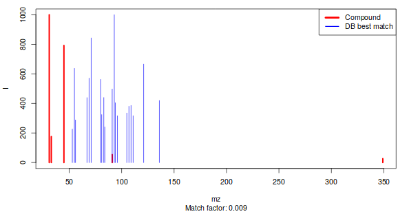
Figure 3: Best match between an experimental pseudospectrum (red) and a database entry (blue)
If an MSP database has been added to the runGC function inputs then the function returns a table where all patterns that have a match with a DB entry are shown with their name. The other non-matching pseudo-spectra will be named UnknownX in the first column of the variableMetadata and dataMatrix.
Once metaMS have created the pseudo-spectra for each unknown compound in each file, we can start the alignment process. This is done by comparing every pseudospectrum to each others in order to group/align similar MS spectra between samples. As a similarity measure, the weighted dot product is used as it is fast, simple, and gives good results (Stein and Scott 1994). The first step in the comparison is based on retention, since a comparison of either retention time or retention index is much faster than a spectral comparison. Since the weighted dot product uses scaled mass spectra, the scaling of the database is done once, and then used in all comparisons. If a pseudo-spectra Y from sample A is similar to pseudo-spectra X in sample B and they have close retention (time or index), the two pseudo-spectra are considered as corresponding to the same compound. This process will create the dataMatrix and variableMetadata outputs, where aligned pseudo-spectra for different samples will belong to the same line in the final variableMetadata and will be considered as Unknown compound X.
Unknowns research
An important aspect of untargeted metabolomics is the definition of unknowns - features that occur repeatedly in a minimum number or fraction of samples (as defined by the min.class.fract and min.class.size parameters in the metaMS settings), but for which no annotation has been found. In metaMS, these unknown features are found by comparing all patterns (i.e. pseudo-spectra which are groups of features) within a certain retention time (or retention index) difference on their spectral characteristics.
If an MSP database has been added to the runGC function inputs, then the function returns a table where all patterns that have a match with a DB entry are shown with their name. The other non-matching pseudo-spectra will be named UnknownX in the first column of the variableMetadata and dataMatrix.
One strenght of metaMS is its ability to use pseudo-spectra (1) for alignment of unknows between samples and (2) to compare unknown experimental pseudo-spectra to previously created in-house spectra databse (in MSP format). By doing so metaMSrunGC function can serve as an annotation tool. You just have to set - “Use Personnal DataBase option” : show and add you in-house database file as input.
The runGC process will always create an MSP file as output (either with only unknown spectra or with a mix of annotated ones and unknowns). That MSP file can be used for database search online (as Golm (J. et al. 2005) and MassBank (Horai et al. 2010)) or locally (NIST MSSEARCH) for NIST search (as shown in the following PDF tutorial.
For large numbers of samples, this process can take quite some time (it scales quadratically), especially if the allowed difference in retention time is large. The result now is a list of two elements: the first is the annotation table that we also saw after the comparison with the database, and the second is a list of pseudo-spectra corresponding to unknowns.
An important aspect of untargeted metabolomics is the definition of unknowns — features that occur repeatedly in a minimum number or fraction of samples (as defined by the min.class.fract and min.class.size parameters in the metaMS settings), but for which no annotation has been found. In metaMS, these unknown features are found by comparing all patterns (i.e. pseudo-spectra which are groups of features) within a certain retention time (or retention index) difference on their spectral characteristics.
Outputs and results
At this stage, all elements are complete: we have the list of pseudo-spectra with an annotation, either as a chemical standard from the database, or an unknown occurring in a sizeable fraction of the injections. The only thing left to do is to calculate relative intensities for the pseudo-spectra, and to put the results in an easy-to-use table. This table consists in two parts. The first part is the information on the “features”, which here are the pseudo-spectra. The second part of the table contains the intensities of these features in the individual injections.
Figure 4: Final table with unknowns and compounds found during the metaMS processus
The first eight lines are the standards, and the next ones are the unknowns that are identified by the pipeline. For each sample, “relative intensities” calculated by metaMS are given.
In the manual interpretation of this kind of data, the intensities of one or two “highly specific” features (called quantifiers) are often used to achieve relative quantitation. In metaMS the reported intensities are calculated differently.
In metaMS, the main measurement for each compound (pseudospectrum) works differently than you might expect. Instead of simply adding up the intensities of different ions belonging to one compound, the package compares what it observes to a “reference model” - think of this as a known fingerprint from a database or a standard sample.
This comparison uses a statistical method called robust linear regression. Here is what this means in simple terms: the software looks for the best scaling factor that makes the observed spectrum match the reference model as closely as possible, while automatically reducing the influence of any unusual or problematic peaks that doesn’t fit the pattern.
This method provides a more reliable estimate that is less affected by random fluctuations in the data and variations in specific peaks or generated by a particularly intense spectra that might throw off simpler calculations.
In practical terms, rather than relying on just one or two ions to quantify a compound (which could be unreliable if those specific ions have problems), metaMS considers the entire ion pattern of the pseudospectrum. It calculates an overall “area” using this regression factor.
This approach minimizes the impact of noisy or problematic peaks while making use of all available information - giving you a more robust and trustworthy measurement for each compound in your GC-MS analysis.
In both cases, the result is a list containing a set of patterns corresponding with the compounds that have been found (either annotated or unknown), the relative intensities of these patterns in the individual annotations, and possibly the xcmsSet object for further inspection. In practice, the runGC function is all that users need to use.
To recap your option 1 journey, here are some questions to check the outcomes of your hands-on:
Question: getting an overview of your GC-MS processing steps
1 - How many known compounds have been detected by metaMS?
The answer is: 8. Here you have to open the param-filepeaktable.tsv and count.
2 - What is the relative intensity of D-Mannitol (6 TMS) in sample alg7?
You should find 74 020 498 in the param-filepeaktable.tsv.
3 - How many Unknowns were detected?
The answer is 198. To be able to see the number of Unknown compounds detected you have to open the param-filepeaktable.tsv file and go to the last line.
Process GC-MS data with a full XCMS workflow (option 2)
This option follows the standard XCMS workflow with GC-MS data as start to obtain in the end a dataMatrix file and its corresponding variableMetadata file. The main difference with the option 1 is that the dataMatrix file will contain individual peaks rather than pseudo-spectra, and the variableMetadata file will contain information about each peak, such as its retention time, m/z, and intensity. No.msp file will be generated in this case, as the peaks are not grouped into pseudo-spectra so the annotation process will be different.
Hands On: Example untargeted GC-MS data processing with the standard XCMS workflow
xcms groupChromPeaks (group) ( Galaxy version 3.12.0+galaxy0) with the following parameters:
param-file“RData file”: xset.merged.RData (output of the xcms findChromPeaks Mergertool job)
“Method to use for grouping”: PeakDensity - peak grouping based on time dimension peak densities
“Bandwidth”: 5.0
“Width of overlapping m/z slices”: 0.5
xcms fillChromPeaks (fillPeaks) ( Galaxy version 3.12.0+galaxy0) with the following parameters:
param-file“RData file”: xset.merged.groupChromPeaks.RData (output of the xcms groupChromPeaks (group)tool job)
In “Peak List”:
“Convert retention time (seconds) into minutes”: Yes
“Number of decimal places for retention time values reported in ions’ identifiers.”: 2
The outputs of this strategy are similar to the ones described in the LC-MS tutotial mentioned previously.
To recap your option 2 journey, here are some questions to check the outcomes of your hands-on:
Question: getting an overview of your GC-MS processing steps
1 - What are the XCMS steps you made in order to obtain your final file RData file?
Here are the different steps made through this tutorial:
(Not with XCMS) import of the data into the Galaxy instance
MSNbase readMSDatatool to read and prepare the MS data for the extraction step
XCMS peak picking with the xcms findChromPeaks (xcmsSet)tool tool
(Not directly XCMS processing, but necessary in the Galaxy tool suit) merge my data into one file with xcms findChromPeaks Mergertool tool
XCMS grouping with the xcms groupChromPeaks (group)tool tool
XCMS integration of missing peaks with xcms fillChromPeaks (fillPeaks)tool tool
2 - What is the complete name of your final RData file?
During each step of the XCMS pre-processing, the name of the file which is processed is completed by the name of the step you used. So, finally your file should be named xset.merged.groupChromPeaks.fillChromPeaks.RData. That means (as seen in the previous question) you have run the findChromPeaks (xcmsSet) step, then a merge, a grouping and finally the filling of missing data.
Verify your data after the pre-processing and clean datasets
The xcms plot chromatogram ( Galaxy version 3.12.0+galaxy3) part allows users to display the TIC (Total Ion Chromatogram) and the BPC (Base Peak Chromatogram).
If you separated your samples into different classes, this tool can constructs TICs and BPCs one class against one class, in a pdf file (see bellow).
The xcms plot chromatogram ( Galaxy version 3.12.0+galaxy3) part allows users to display the TIC (Total Ion Chromatogram) and the BPC (Base Peak Chromatogram).
When you have processed all or only needed steps described before, you can continue the processing of your data with statistics or annotation tools.
Don’t forget to always check your files’ format for compatibility with further analysis!
The pre-processing part of this analysis can be quite time-consuming, and already corresponds to quite a few number of steps, depending of your analysis. If you plan to proceed with further steps in Galaxy (statistics for example), we highly recommend, at this step of the GC-MS workflow, to split your analysis by beginning a new Galaxy history with only the files you need for further steps (that would be the final .tsv matrices - sampleMetadata, variableMetadata, dataMatrix - and the .msp spectral database). This will help you in limiting the chance to select the wrong dataset in further analysis, and bring a little tidiness for future review of your analysis process. This would also enable you to make alternative extractions in the future (by adjusting peak picking parameters) in the same history, without drowning your statistical analysis steps far bellow.
To begin a new history with the files from your current history, you can use the functionality ‘copy dataset’ and copy it into a new history.
There 3 ways to copy datasets between histories
From the original history
Click on the galaxy-gear icon which is on the top of the list of datasets in the history panel
Click on Copy Datasets
Select the desired files
Give a relevant name to the “New history”
Validate by ‘Copy History Items’
Click on the new history name in the green box that have just appear to switch to this history
Using the galaxy-columnsShow Histories Side-by-Side
Click on the galaxy-dropdown dropdown arrow top right of the history panel (History options)
Click on galaxy-columnsShow Histories Side-by-Side
If your target history is not present
Click on ‘Select histories’
Click on your target history
Validate by ‘Change Selected’
Drag the dataset to copy from its original history
Drop it in the target history
From the target history
Click on User in the top bar
Click on Datasets
Search for the dataset to copy
Click on its name
Click on Copy to current History
You may have notice that the XCMS tools generate output names that contain the different XCMS steps you used, allowing easy traceability while browsing your history. Hence, when begining further processing steps (as statistics), we highly recommend you (in particular if you have used the option 2) to first rename your datasets with something short, e.g. “dataMatrix”, “variableMetadata”, or anything not too long that you may find convenient.
Click on the galaxy-pencilpencil icon for the dataset to edit its attributes
In the central panel, change the Name field
Click the Save button
Warning: Be careful of the file format
During each step of pre-processing, your dataset has its formats changed and can have also its name changed. To be able to proceed with GC-MS processing with metaMS, you need to identify which datasets can be used with which tool. For example to be able to use runGC function you need to have an RData object which is at least merged (output from xcms findChromPeaks Mergertool).
After following the option 1 steps you obtained tabular files that can be used in a large variety of analyses, as well as an MSP file (if option 1 was used). Always check the format needed for further tools, as these format are ‘text format’ but with characteristics that may matter in further steps.
With option 2, if you want to process your data with XCMS or other tools you may also have to align them with xcms groupChromPeaks (group)tool. It means that you should have at least a file named xset.merged.RData to be able to continue XCMS processing.
Stein, S. E., and D. R. Scott, 1994 Optimization and testing of mass spectral library search algorithms for compound identification. Journal of the American Society for Mass Spectrometry 5: 859–866. 10.1016/1044-0305(94)87009-8
Smith, C. A., E. J. Want, G. O’Maille, R. Abagyan, and G. Siuzdak, 2006 XCMS: Processing Mass Spectrometry Data for Metabolite Profiling Using Nonlinear Peak Alignment, Matching, and Identification. Analytical Chemistry 78: 779–787. 10.1021/ac051437y
Dittami, S. M., A. Gravot, S. Goulitquer, S. Rousvoal, A. F. Peters et al., 2012 Towards deciphering dynamic changes and evolutionarymechanisms involved in the adaptation to low salinities inEctocarpus(brown algae). The Plant Journal 71: 366–377. 10.1111/j.1365-313X.2012.04982.x
Gatto, L., and K. S. Lilley, 2012 MSnbase-an R/Bioconductor package for isobaric tagged mass spectrometry data visualization, processing and quantitation. Bioinformatics 28: 288–289. 10.1093/bioinformatics/btr645
Wehrens, R., G. Weingart, and F. Mattivi, 2014 metaMS: An open-source pipeline for GC-MS-based untargeted metabolomics. Journal of Chromatography B 966: 109–116. 10.1016/j.jchromb.2014.02.051
Gatto, L., S. Gibb, and J. Rainer, 2020 MSnbase, efficient and elegant R-based processing and visualization of raw mass spectrometry data. Journal of Proteome Research 20: 1063–1069. 10.1021/acs.jproteome.0c00313
Misra, B. B., 2021 New software tools, databases, and resources in metabolomics: updates from 2020. Metabolomics 17: 49. 10.1007/s11306-021-01796-1 ISBN: 0123456789
Feedback
Did you use this material as an instructor? Feel free to give us feedback on how it went.
Did you use this material as a learner or student? Click the form below to leave feedback.
Hiltemann, Saskia, Rasche, Helena et al., 2023 Galaxy Training: A Powerful Framework for Teaching! PLOS Computational Biology 10.1371/journal.pcbi.1010752
Batut et al., 2018 Community-Driven Data Analysis Training for Biology Cell Systems 10.1016/j.cels.2018.05.012
@misc{metabolomics-gcms,
author = "Julien Saint-Vanne and Yann Guitton",
	title = "Mass spectrometry: GC-MS analysis with the metaMS package (Galaxy Training Materials)",
	year = "",
	month = "",
	day = "",
	url = "\url{https://training.galaxyproject.org/training-material/topics/metabolomics/tutorials/gcms/tutorial.html}",
	note = "[Online; accessed TODAY]"
}
@article{Hiltemann_2023,
	doi = {10.1371/journal.pcbi.1010752},
	url = {https://doi.org/10.1371%2Fjournal.pcbi.1010752},
	year = 2023,
	month = {jan},
	publisher = {Public Library of Science ({PLoS})},
	volume = {19},
	number = {1},
	pages = {e1010752},
	author = {Saskia Hiltemann and Helena Rasche and Simon Gladman and Hans-Rudolf Hotz and Delphine Larivi{\`{e}}re and Daniel Blankenberg and Pratik D. Jagtap and Thomas Wollmann and Anthony Bretaudeau and Nadia Gou{\'{e}} and Timothy J. Griffin and Coline Royaux and Yvan Le Bras and Subina Mehta and Anna Syme and Frederik Coppens and Bert Droesbeke and Nicola Soranzo and Wendi Bacon and Fotis Psomopoulos and Crist{\'{o}}bal Gallardo-Alba and John Davis and Melanie Christine Föll and Matthias Fahrner and Maria A. Doyle and Beatriz Serrano-Solano and Anne Claire Fouilloux and Peter van Heusden and Wolfgang Maier and Dave Clements and Florian Heyl and Björn Grüning and B{\'{e}}r{\'{e}}nice Batut and},
	editor = {Francis Ouellette},
	title = {Galaxy Training: A powerful framework for teaching!},
	journal = {PLoS Comput Biol}
}
Funding
These individuals or organisations provided funding support for the development of this resource
Questions:

 Open image in new tab
Open image in new tab
 Open image in new tab
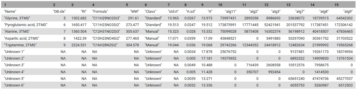 Open image in new tab
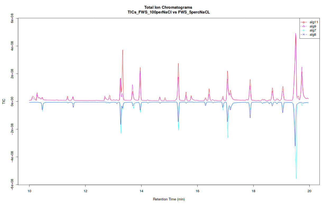 Open image in new tab