Can I predict QC-based mass spectra starting from SMILES?
How can I run those computationally heavy predictions?
Can I take into account different conformers?
Objectives:
To prepare structure-data format (SDF) files for further operations analysis, starting from chemical structure descriptors in simplified molecular-input line-entry system (SMILES) format.
To generate 3D conformers and optimise them using semi-empirical quantum mechanical (SQM) methods.
To produce simulated mass spectra for a given molecule in MSP (text based) format.
Mass spectrometry (MS) is a powerful analytical technique used in many fields, including proteomics, metabolomics, drug discovery and many more areas relying on compound identifications. Even though nowadays MS is a standard and popular method, there are many compounds which lack experimental spectra. In those cases, predicting mass spectra from the chemical structure can reveal useful information, help in compound identification and expand the spectral databases, improving the accuracy and efficiency of database search. [Zhu and Jonas 2023, Allen et al. 2016].
There have been several methods developed to predict mass spectra, which can be classified as either first-principles physical-based simulation or data-driven statistical methods [Zhu and Jonas 2023]. To the first category we can assign purely statistical theories (quasi-equilibrium theory (QET) or Rice–Ramsperger–Kassel–Marcus (RRKM) theories) [Vetter 1994], as well as QCxMS [Koopman and Grimme 2021] and semiempirical GFNn-xTB [Koopman and Grimme 2019] which use Born–Oppenheimer molecular dynamics (MD) combined with fragmentation pathways. Data-driven statistical methods - forming the second category - reach back to 1960s when the DENDRAL project (using rule-based heuristic programming) was started by early artificial intelligence (AI) scientists [Lindsay et al. 1980]. More recently, CFM-ID has been introduced [Allen et al. 2014, Allen et al. 2014, Allen et al. 2016, Djoumbou-Feunang et al. 2019, Wang et al. 2020], which uses rule-based fragmentation and employs machine learning methods. Current advancements in machine learning led to recent work using deep neural networks that allow predicting spectra from molecular graphs or fingerprints [Wei et al. 2019].
You will be able to check out how QCxMS works in practice since we are going to use Galaxy tool suite based on this method [Grimme 2013, Bauer and Grimme 2014, Bauer and Grimme 2016, Koopman and Grimme 2021]. Beforehand, we will generate conformers of the query molecule with RDKit and we will use xTB for molecular optimisation [Bannwarth et al. 2020].
But first things first, let’s get some toy data to play with and crack on!
Question
What does QCEIMS stand for?
With a little knowledge of chemistry, you’ll be able to work it out yourself!
Look at the acronym in the following way: QC-EI-MS.
QC = quantum chemical
EI = electron ionisation
MS = mass spectrometry
Hence QCEIMS = quantum-chemical electron ionisation mass spectrometry
QCxMS is a successor of QCEIMS, where the EI part is replaced by x to take into account other ionisation methods and improve the applicability of the program. In QCEIMS, EI stands for electron ionisation, while in QCxMS, x refers to EI or CID (collision-induced dissociation) [Koopman and Grimme 2021]. Currently, only EI simulations are supported - using CID with the Galaxy tool wrappers is still under development.
Importing data and pre-processing
In this tutorial, you can choose whether you want to predict the mass spectrum for one molecule only, or if you want to do it for multiple molecules at once. The pre-processing steps will slightly differ depending on your choice. If you are completing this tutorial just to see how the QCxMS tools work, feel free to follow the instructions for one molecule to skip some pre-processing steps.
In both cases, we start from molecule’s SMILES, and then we convert it to SDF, so if you already have SDF files to work with, simply jump in the relevant place in the workflow and carry on from there.
SMILES (.smi) - the simplified molecular-input line-entry system (SMILES) is a specification in the form of a line notation for describing the structure of a chemical species using short ASCII strings. It is a linear text format which can describe the connectivity and chirality of a molecule [Weininger 1988]. Even though many different forms of SMILES exist, the differences are not relevant for us in this application.
Figure 1: A quick explanation of the SMILES system.
Image credit: Helge Hecht, License: MIT
Hands-on: Choose Your Own Tutorial
This is a 'Choose Your Own Tutorial' (CYOT) section (also known as 'Choose Your Own Analysis' (CYOA)), where you can select between multiple paths. Click one of the buttons below to select how you want to follow the tutorial
Choose below if you just want to follow the pipeline for prediting the spectrum for only one molecule or multiple molecules at once!
Upload data onto Galaxy
Working on a single molecule means that we will work on a dataset and not on a collection of datasets. To simulate the spectrum, we will use ethanol (C2H5 OH) as an example, but you can choose any other molecule that you want, but be aware that the more complex structure you choose, the more time it will take to complete the analysis since the workflow involves generating conformers, semiempirical methods and molecular optimisation.
We will simply start with molecule’s SMILES.
You have three options for uploading the data. The first two - importing via history and Zenodo link will give a file specific to this tutorial, while the last one – “Paste data uploader” gives you more flexibility in terms of the compounds you would like to test with this workflow.
Hands On: Option 1: Data upload - Import history
You can simply import this history with the input file.
Open the link to the shared history
Click on the Import this history button on the top left
Enter a title for the new history
Click on Copy History
Renamegalaxy-pencil the history to your name of choice.
Hands On: Option 2: Data upload - Add to history via Zenodo
Click galaxy-uploadUpload at the top of the activity panel
Select galaxy-wf-editPaste/Fetch Data
Paste the link(s) into the text field
Press Start
Close the window
Hands On: Option 3: Data Upload - paste data
Create a new history for this tutorial
Click galaxy-uploadUpload Data at the top of the tool panel
Select galaxy-wf-editPaste/Fetch Data at the bottom
Paste the SMILES into the text field:
CCO
Change Type from “Auto-detect” to smi
Press Start and Close the window
You can then rename the dataset as you wish (here we use ethanol_SMILES)
Check that the datatype is smi.
Click on the galaxy-pencilpencil icon for the dataset to edit its attributes
In the central panel, click galaxy-chart-select-dataDatatypes tab on the top
In the galaxy-chart-select-dataAssign Datatype, select smi from “New Type” dropdown
Tip: you can start typing the datatype into the field to filter the dropdown menu
Click the Save button
SMILES to SDF
Hands On: Convert SMILES to SDF
Compound conversion ( Galaxy version 3.1.1+galaxy0) with the following parameters:
param-file“Molecular input file”: ethanol_SMILES (your SMILES dataset from your history)
“Output format”: MDL MOL format (sdf, mol)
“Append the specified text after each molecule title”: ethanol
We now have an SDF file, containing the atoms’ coordinates and the investigated molecule’s name.
3D Conformer generation & optimization
Generate conformers
The next step involves generating three-dimensional (3D) conformers for our molecule. It crteaes the actual 3D topology of the molecule based on electromagnetic forces. This process might seem trivial for very small and simplistic (meaning no complex structure) molecules, but this can be more challenging for larger molecules with a more flexible geometry. This concerns for example P containing biomolecules, where P often forms a rotational center of the molecule. The number of conformers to generate can be specified as an input parameter, with a default value of 1 if not provided. This process is crucial for exploring the possible shapes and energies that a molecule can adopt. The output of this step is a file containing the generated 3D conformers.
Conformers are different spatial arrangements of a molecule that result from rotations around single bonds. They have different potential energies and hence some are more favourable (local minima on the potential energy surface) than others.
Generate conformers ( Galaxy version 1.1.4+galaxy0) with the following parameters:
param-file“Input file”: output of Convert to sdftool
“Number of conformers to generate”: 1
Now - once again format conversion! This time we will convert the generated conformers from the SDF format to Cartesian coordinate (XYZ) format. The XYZ format lists the atoms in a molecule and their respective 3D coordinates, which is a common format used in computational chemistry for further processing and analysis.
Hands On: Molecular Format Conversion
Compound conversion ( Galaxy version 3.1.1+galaxy0) with the following parameters:
param-file“Molecular input file”: output (sdf) of Generate conformerstool
“Output format”: XYZ cartesian coordinates format
“Add hydrogens appropriate for pH”: 7.0
Check that the datatype is xyz. If it’s not, just change it – below is the tip how to do it.
Click on the galaxy-pencilpencil icon for the dataset to edit its attributes
In the central panel, click galaxy-chart-select-dataDatatypes tab on the top
In the galaxy-chart-select-dataAssign Datatype, select xyz from “New Type” dropdown
Tip: you can start typing the datatype into the field to filter the dropdown menu
Click the Save button
Molecular optimization
As shown in the image in the detailsDetails box above, different conformers have different energies. Therefore, our next step will optimize the geometry of the molecules to find the lowest energy conformation. This is crucial to achieve convergence in the next steps. If the input geometry for the QCxMS method is too crude, the ground state neutral run will not converge and we won’t be able to sample the geometry to calculate individual trajectories. We will perform semi-empirical optimization on the molecules using the Extended Tight-Binding (xTB) method. The level of optimization accuracy to be used can be specified as an input parameter, “Optimization Levels”. The default quantum chemical method is GFN2-xTB.
Hands On: Molecular optimisation with xTB
xtb molecular optimization ( Galaxy version 6.6.1+galaxy1) with the following parameters:
param-file“Atomic coordinates file”: output of Convert to xyztool)
“Optimization Levels”: tight
“Keep molecule name”: galaxy-toggleYes
QCxMS Spectra Prediction
Neutral and production runs
Finally, let’s predict the spectra for our molecule. As mentioned, we will use QCxMS for this purpose. First, we need to prepare the necessary input files for the QCxMS production runs. These files are required for running the QCxMS simulations, which will predict the mass spectrum of the molecule. This step typically formats the optimized molecular data into a format that can be used for the production simulations. This step performs the ground state calculations. The resulting geometry trajectory is then sampled and one representation is used for each trajectory.
Hands On: QCxMS neutral run
QCxMS neutral run ( Galaxy version 5.2.1+galaxy3) with the following parameters:
param-file“Molecule 3D structure [.xyz]”: output of xtb molecular optimizationtool
“QC Method”: GFN2-xTB
The outputs of the above step are as follows:
.in output: Input file for the QCxMS production run
.start output: Start file for the QCxMS production run
.xyz output: Cartesian coordinate file for the QCxMS production run
We can now use those files as input for the next tool which calculates the mass spectra using QCxMS. This simulation generates .res files, which contain the raw results of the mass spectra calculations. These results are essential for predicting how the molecules will appear in mass spectrometry experiments.
Hands On: QCxMS production run
QCxMS production run ( Galaxy version 5.2.1+galaxy3) with the following parameters:
param-collectionDataset collection“in files [.in]”: input in files generated by QCxMS neutral runtool
It might be the case that some runs might have failed, therefore it is crucial to filter out any failed runs from the dataset to ensure only successful results are processed further. This step is important to maintain the integrity and quality of the data being analyzed in subsequent steps. The output is a file containing only the successful mass spectra results.
Hands On: Filter failed datasets
Filter failed datasets with the following parameters:
param-collection“Input Collection”: res files generated by QCxMS (output of QCxMS production runtool )
Get MSP spectra
The filtered collection contains .res files from the QCxMS production run. This final step converts the .res files into simulated mass spectra in MSP (Mass Spectrum Peak) file format. The MSP format is widely used for storing and sharing mass spectrometry data, enabling easy comparison and analysis of the results, for example by comparing the spectra using the matchms package.
Hands On: QCxMS get MSP results
QCxMS get results ( Galaxy version 5.2.1+galaxy2) with the following parameters:
param-file“Molecule 3D structure [.xyz]”: Convert to xyz (output of Compound conversiontool)
“res files [.res]”: output of Filter failed datasetstool (if the collection doesn’t appear in the drop-down list, simply drag and drop it from the history panel to the input box)
MSP (Mass Spectrum Peak) file is a text file structured according to the NIST MSSearch spectra format. MSP is one of the generally accepted formats for mass spectral libraries (or collections of unidentified spectra, so called spectral archives), and it is compatible with lots of spectra processing programmes (MS-DIAL, NIST MS Search, AMDIS, matchms, etc.). It can contain one or more mass spectra, these are split by an empty line. The individual spectra essentially consist of two sections: metadata (such as name, spectrum type, ion mode, retention time, and the number of m/z peaks) and peaks, consisting of m/z and intensity tuples.
You can now dataset-save download the MSP file and open it in your spectra processing software for further investigation!
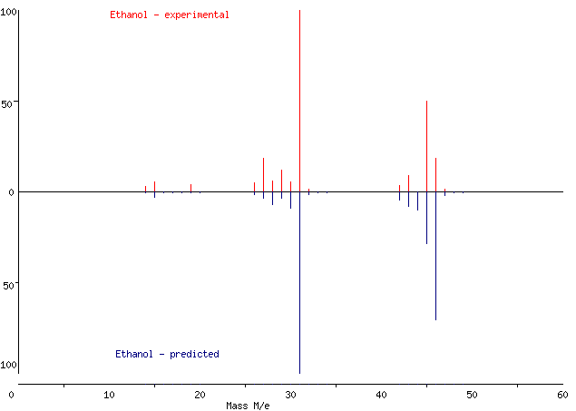
To give you some insight into how well QCxMS can perform, below is the mass spectrum of ethanol resulting from our workflow compared with an experimental spectrum. Both spectra were compiled using an online mass spectrum generator which requires only m/z values and intensities – so the values that you can get from our MSP file! As you can see, the predicted peaks nicely correspond to experimental ones. But be careful - there might be slight deviations for molecules with more structural complexity!
Figure 3: Comparison between experimental (upper panel) and predicted (lower panel) mass spectra of ethanol.
Conclusion
trophy Well done, you’ve simulated the mass spectrum! You might want to consult your results with the key history. If you would like to process multiple molecules at once, you can simply use the workflow or move to “Predict MS for multiple molecules at once” tab of this tutorial to learn how the pipeline differs from the one that we’ve just covered.
Upload data onto Galaxy
We will work on two simple molecules – ethanol (C2H5 OH) and ethylene (C2H4). Of course, you might add more and choose any other molecules that you want, but be aware that the more complex structure you choose, the more time it will take to complete the analysis since the workflow involves generating conformers, semiempirical methods and molecular optimisation.
We will start with a table with the first column being molecule names and the second one – corresponding SMILES.
You have three options for uploading the data. The first two - importing via history and Zenodo link will give a file specific to this tutorial, while the last one – “Paste data uploader” gives you more flexibility in terms of the compounds you would like to test with this workflow.
Hands On: Option 1: Data upload - Import history
You can simply import this history with the input table.
Open the link to the shared history
Click on the Import this history button on the top left
Enter a title for the new history
Click on Copy History
Renamegalaxy-pencil the history to your name of choice.
Hands On: Option 2: Data upload - Add to history via Zenodo
Click galaxy-uploadUpload at the top of the activity panel
Select galaxy-wf-editPaste/Fetch Data
Paste the link(s) into the text field
Press Start
Close the window
Hands On: Option 3: Data Upload - paste data
Create a new history for this tutorial
Click galaxy-uploadUpload Data at the top of the tool panel
Select galaxy-wf-editPaste/Fetch Data at the bottom
Paste the contents into the text field, separated by space. First, enter the name of the molecule, then its SMILES. Please note that we are not using headers here. For this tutorial, we’ll use the example of ethanol and ethylene, but feel free to use your own examples.
ethanol CCO
ethylene C=C
Change Type from “Auto-detect” to tabular
Find the gear symbol (galaxy-gear), deselect any ticked options and select only (galaxy-gear) Convert spaces to tabs
Press Start and Close the window
You can then rename the dataset as you wish.
Check that the datatype is tabular.
Click on the galaxy-pencilpencil icon for the dataset to edit its attributes
In the central panel, click galaxy-chart-select-dataDatatypes tab on the top
In the galaxy-chart-select-dataAssign Datatype, select tabular from “New Type” dropdown
Tip: you can start typing the datatype into the field to filter the dropdown menu
Click the Save button
Input pre-processing
Once your dataset is uploaded, we can do some simple pre-processing to prepare the file for downstream analysis. Let’s start with ‘cutting’ the table into two columns – one with SMILES, the other with the molecule name – and then separating each entry to create a dataset collection, followed by parsing out the text information.
Hands On: Cutting out name column
Advanced Cut ( Galaxy version 9.3+galaxy1) with the following parameters:
param-file“File to cut”: the tabular file in your history with the compound name and SMILES
“Operation”: Keep
“Cut by”: fields
“Delimited by”: Tab
“Is there a header for the data’s columns”: No
“List of Fields”: Column: 1
You can now rename the resulting dataset or just add a tag in order not to confuse it with subsequent outputs:
galaxy-tags Add tag: #names
Datasets can be tagged. This simplifies the tracking of datasets across the Galaxy interface. Tags can contain any combination of letters or numbers but cannot contain spaces.
To tag a dataset:
Click on the dataset to expand it
Click on Add Tagsgalaxy-tags
Add tag text. Tags starting with # will be automatically propagated to the outputs of tools using this dataset (see below).
Press Enter
Check that the tag appears below the dataset name
Tags beginning with # are special!
They are called Name tags. The unique feature of these tags is that they propagate: if a dataset is labelled with a name tag, all derivatives (children) of this dataset will automatically inherit this tag (see below). The figure below explains why this is so useful. Consider the following analysis (numbers in parenthesis correspond to dataset numbers in the figure below):
a set of forward and reverse reads (datasets 1 and 2) is mapped against a reference using Bowtie2 generating dataset 3;
dataset 3 is used to calculate read coverage using BedTools Genome Coverageseparately for + and - strands. This generates two datasets (4 and 5 for plus and minus, respectively);
datasets 4 and 5 are used as inputs to Macs2 broadCall datasets generating datasets 6 and 8;
datasets 6 and 8 are intersected with coordinates of genes (dataset 9) using BedTools Intersect generating datasets 10 and 11.
Now consider that this analysis is done without name tags. This is shown on the left side of the figure. It is hard to trace which datasets contain “plus” data versus “minus” data. For example, does dataset 10 contain “plus” data or “minus” data? Probably “minus” but are you sure? In the case of a small history like the one shown here, it is possible to trace this manually but as the size of a history grows it will become very challenging.
The right side of the figure shows exactly the same analysis, but using name tags. When the analysis was conducted datasets 4 and 5 were tagged with #plus and #minus, respectively. When they were used as inputs to Macs2 resulting datasets 6 and 8 automatically inherited them and so on… As a result it is straightforward to trace both branches (plus and minus) of this analysis.
Hands On: Creating dataset collection (molecule name)
Split file to dataset collection ( Galaxy version 0.5.2) with the following parameters:
param-file“Select the file type to split”: Tabular
“Tabular file to split”: output of Advanced Cuttool (with #names tag)
“Number of header lines to transfer to new files”: 0
“Split by row or by a column?”: By row
“Specify number of output files or number of records per file?”: Number of records per file (‘chunk mode’)
“Chunk size”: 1
“Base name for new files in collection”: split_file
“Method to allocate records to new files”: Maintain record order
Hands On: Parsing out name info
Parse parameter value with the following parameters:
“Input file containing parameter to parse out of”: * click on param-collectionDataset collection and select output of Split filetool
“Select type of parameter to parse”: Text
“Remove newlines ?”: galaxy-toggleYes
If you have any problems with accessing Parse parameter value tool, you can open the tool directly using a given link.
We will repeat the first two steps, but processing SMILES this time.
Hands On: Cutting out SMILES column
Advanced Cut ( Galaxy version 9.3+galaxy1) with the following parameters:
param-file“File to cut”: the tabular file in your history with the compound name and SMILES
“Operation”: Keep
“Cut by”: fields
“Delimited by”: Tab
“Is there a header for the data’s columns”: No
“List of Fields”: Column: 2
You can now rename the resulting dataset or just add a tag in order not to confuse it with subsequent outputs:
galaxy-tags Add tag: #SMILES
Datasets can be tagged. This simplifies the tracking of datasets across the Galaxy interface. Tags can contain any combination of letters or numbers but cannot contain spaces.
To tag a dataset:
Click on the dataset to expand it
Click on Add Tagsgalaxy-tags
Add tag text. Tags starting with # will be automatically propagated to the outputs of tools using this dataset (see below).
Press Enter
Check that the tag appears below the dataset name
Tags beginning with # are special!
They are called Name tags. The unique feature of these tags is that they propagate: if a dataset is labelled with a name tag, all derivatives (children) of this dataset will automatically inherit this tag (see below). The figure below explains why this is so useful. Consider the following analysis (numbers in parenthesis correspond to dataset numbers in the figure below):
a set of forward and reverse reads (datasets 1 and 2) is mapped against a reference using Bowtie2 generating dataset 3;
dataset 3 is used to calculate read coverage using BedTools Genome Coverageseparately for + and - strands. This generates two datasets (4 and 5 for plus and minus, respectively);
datasets 4 and 5 are used as inputs to Macs2 broadCall datasets generating datasets 6 and 8;
datasets 6 and 8 are intersected with coordinates of genes (dataset 9) using BedTools Intersect generating datasets 10 and 11.
Now consider that this analysis is done without name tags. This is shown on the left side of the figure. It is hard to trace which datasets contain “plus” data versus “minus” data. For example, does dataset 10 contain “plus” data or “minus” data? Probably “minus” but are you sure? In the case of a small history like the one shown here, it is possible to trace this manually but as the size of a history grows it will become very challenging.
The right side of the figure shows exactly the same analysis, but using name tags. When the analysis was conducted datasets 4 and 5 were tagged with #plus and #minus, respectively. When they were used as inputs to Macs2 resulting datasets 6 and 8 automatically inherited them and so on… As a result it is straightforward to trace both branches (plus and minus) of this analysis.
Split file to dataset collection ( Galaxy version 0.5.2) with the following parameters:
param-file“Select the file type to split”: Tabular
“Tabular file to split”: output of the latest Advanced Cuttool (higher number in your history, with #SMILES tag)
“Number of header lines to transfer to new files”: 0
“Split by row or by a column?”: By row
“Specify number of output files or number of records per file?”: Number of records per file (‘chunk mode’)
“Chunk size”: 1
“Base name for new files in collection”: split_file
“Method to allocate records to new files”: Maintain record order
Check that the datatype is smi. If it’s not, just change it!
Click on the galaxy-pencilpencil icon for the dataset to edit its attributes
In the central panel, click galaxy-chart-select-dataDatatypes tab on the top
In the galaxy-chart-select-dataAssign Datatype, select smi from “New Type” dropdown
Tip: you can start typing the datatype into the field to filter the dropdown menu
Click the Save button
Now, onto format conversion. Let’s convert our SMILES to SDF (Structure Data File) and append the molecule’s name that we have already extracted.
Hands On: Convert SMILES to SDF
Compound conversion ( Galaxy version 3.1.1+galaxy0) with the following parameters:
“Molecular input file”: click on param-collectionDataset collection and select output of Split filetool on SMILES
“Output format”: MDL MOL format (sdf, mol)
Another parameter of this tool, “Append the specified text after each molecule title”, allows you to add name of the molecule to the title of the generated file.
If you are working on a single molecule file, you can simply type the name of that compound into the parameter box.
However, if your input is a collection of SMILES (like in this case), then you have to add the names (output of Parse parameter valuetool) at the level of the workflow editor.
We now have two SDF files, each containing the coordinates of the atoms and the name of the investigated molecule. Let’s combine them to make life easier and work on just one file.
Hands On: Concatenating the files
Concatenate datasets tail-to-head (cat) ( Galaxy version 9.3+galaxy1) with the following parameters:
param-file“Datasets to concatenate”:
if nothing pops up when you click on param-collectionDataset collection, then click on “switch to column select”
from the datasets list, find the output of Compound conversiontool (should have the highest number in your history) and select it
workflow-run Run tool!
3D Conformer generation & optimization
Generate conformers
The next step involves generating three-dimensional (3D) conformers for each molecule from the generated SDF. It crteaes the actual 3D topology of the molecules based on electromagnetic forces. This process might seem trivial for very small and simplistic (meaning no complex structure) molecules, but this can be more challenging for larger molecules with a more flexible geometry. This concerns for example P containing biomolecules, where P often forms a rotational center of the molecule. The number of conformers to generate can be specified as an input parameter, with a default value of 1 if not provided. This process is crucial for exploring the possible shapes and energies that a molecule can adopt. The output of this step is a file containing the generated 3D conformers.
Conformers are different spatial arrangements of a molecule that result from rotations around single bonds. They have different potential energies and hence some are more favourable (local minima on the potential energy surface) than others.
Generate conformers ( Galaxy version 1.1.4+galaxy0) with the following parameters:
param-file“Input file”: output of Concatenate datasetstool
“Number of conformers to generate”: 1
Now - once again format conversion! This time we will convert the generated conformers from the SDF format to Cartesian coordinate (XYZ) format. The XYZ format lists the atoms in a molecule and their respective 3D coordinates, which is a common format used in computational chemistry for further processing and analysis.
Hands On: Molecular Format Conversion
Compound conversion ( Galaxy version 3.1.1+galaxy0) with the following parameters:
param-file“Molecular input file”: output of Generate conformerstool
“Output format”: XYZ cartesian coordinates format
“Split multi-molecule files into a collection”: galaxy-toggleYes
“Add hydrogens appropriate for pH”: 7.0
Check that the datatype is xyz. If it’s not, just change it!
Click on the galaxy-pencilpencil icon for the dataset to edit its attributes
In the central panel, click galaxy-chart-select-dataDatatypes tab on the top
In the galaxy-chart-select-dataAssign Datatype, select xyz from “New Type” dropdown
Tip: you can start typing the datatype into the field to filter the dropdown menu
Click the Save button
Molecular optimization
As shown in the image in the detailsDetails box above, different conformers have different energies. Therefore, our next step will optimize the geometry of the molecules to find the lowest energy conformation. This is crucial to achieve convergence in the next steps. If the input geometry for the QCxMS method is too crude, the ground state neutral run will not converge and we won’t be able to sample the geometry to calculate individual trajectories. We will perform semi-empirical optimization on the molecules using the Extended Tight-Binding (xTB) method. The level of optimization accuracy to be used can be specified as an input parameter, “Optimization Levels”. The default quantum chemical method is GFN2-xTB.
Hands On: Molecular optimisation with xTB
xtb molecular optimization ( Galaxy version 6.6.1+galaxy1) with the following parameters:
“Atomic coordinates file”: click on param-collectionDataset collection and select Prepared ligands (output of Compound conversiontool)
“Optimization Levels”: tight
“Keep molecule name”: galaxy-toggleYes
QCxMS Spectra Prediction
Neutral and production runs
Finally, let’s predict the spectra for our molecules. As mentioned, we will use QCxMS for this purpose. First, we need to prepare the necessary input files for the QCxMS production runs. These files are required for running the QCxMS simulations, which will predict the mass spectra of the molecules. This step typically formats the optimized molecular data into a format that can be used for the production simulations. This step performs the ground state calculations. The resulting geometry trajectory is then sampled and one representation is used for each trajectory.
Hands On: QCxMS neutral run
QCxMS neutral run ( Galaxy version 5.2.1+galaxy3) with the following parameters:
“Molecule 3D structure [.xyz]”: click on param-collectionDataset collection and select output of xtb molecular optimizationtool
“QC Method”: GFN2-xTB
The outputs of the above step are as follows:
.in output: Input file for the QCxMS production run
.start output: Start file for the QCxMS production run
.xyz output: Cartesian coordinate file for the QCxMS production run
We can now use those files as input for the next tool which calculates the mass spectra for each molecule using QCxMS (Quantum Chemistry and Mass Spectrometry). This simulation generates .res files, which contain the raw results of the mass spectra calculations. These results are essential for predicting how the molecules will appear in mass spectrometry experiments.
Hands On: QCxMS production run
QCxMS production run ( Galaxy version 5.2.1+galaxy3) with the following parameters:
param-collectionDataset collection“in files [.in]”: input in files generated by QCxMS neutral runtool
It might be the case that some runs might have failed, therefore it is crucial to filter out any failed runs from the dataset to ensure only successful results are processed further. This step is important to maintain the integrity and quality of the data being analyzed in subsequent steps. The output is a file containing only the successful mass spectra results.
Hands On: Filter failed datasets
Filter failed datasets with the following parameters:
param-collection“Input Collection”: output of QCxMS production runtool
Get MSP spectra
The filtered collection contains .res files from the QCxMS production run. This final step converts the .res files into simulated mass spectra in MSP (Mass Spectrum Peak) file format. The MSP format is widely used for storing and sharing mass spectrometry data, enabling easy comparison and analysis of the results, for example by comparing the spectra using the matchms package.
Hands On: QCxMS get MSP results
QCxMS get results ( Galaxy version 5.2.1+galaxy2) with the following parameters:
“Molecule 3D structure [.xyz]”: click on param-collectionDataset collection and select Prepared ligands (output of Compound conversiontool)
param-file“res files [.res]”: output of Filter failed datasetstool (if the collection doesn’t appear in the drop-down list, simply drag and drop it from the history panel to the input box)
The output of this step is a collection of two MSP files - one per each molecule. However, if you want, you can combine those two into one MSP file.
Hands On: Combine MSP files into one
Concatenate datasets tail-to-head (cat) ( Galaxy version 9.3+galaxy1) with the following parameters:
param-file“Datasets to concatenate”:
if nothing pops up when you click on param-collectionDataset collection, then click on “switch to column select”
from the datasets list, find the output of QCxMS get resultstool (should be the latest output dataset) and select it
workflow-run Run tool!
MSP (Mass Spectrum Peak) file is a text file structured according to the NIST MSSearch spectra format. MSP is one of the generally accepted formats for mass spectral libraries (or collections of unidentified spectra, so called spectral archives), and it is compatible with lots of spectra processing programmes (MS-DIAL, NIST MS Search, AMDIS, matchms, etc.). It can contain one or more mass spectra, these are split by an empty line. The individual spectra essentially consist of two sections: metadata (such as name, spectrum type, ion mode, retention time, and the number of m/z peaks) and peaks, consisting of m/z and intensity tuples.
You can now dataset-save download the MSP file and open it in your spectra processing software for further investigation!
To give you some insight into how well QCxMS can perform, below is the mass spectrum of ethanol resulting from our workflow compared with experimental spectrum. Both spectra were compiled using an online mass spectrum generator which requires only m/z values and intensities – so the values that you can get from our MSP file! As you can see, the predicted peaks nicely correspond to experimental ones. But be careful - there might be slight deviations for molecules with more structural complexity!
Figure 5: Comparison between experimental (upper panel) and predicted (lower panel) mass spectra of ethanol.
Conclusion
trophy Well done, you’ve simulated mass spectra! You might want to consult your results with the key history or use the workflow associated with this tutorial.
The prediction of mass spectra might be very useful, particularly for compounds that lack experimental data. Simulating the spectra can also save time and resources. This field has been developing quite rapidly, and recent advancements in new algorithms and packages have led to more and more accurate results. However, one cannot forget that this kind of software should be used to deepen our chemical understanding of the structures of studied compounds and not as a replacement for practical experiments.
You've Finished the Tutorial
Please also consider filling out the Feedback Form as well!
Key points
Galaxy provides access to high-performance computing (HPC) resources and hence allows the use of semi-empirical quantum mechanical (SQM) methods and in silico prediction of QC-based mass spectra.
The shown workflow allows to simulate mass spectra of a molecule starting from its SMILES.
The xTB package is based on a SQM method to optimise the geometry of the generated conformers.
The QCxMS tool suite performs quantum chemistry calculations to simulate mass spectra.
Frequently Asked Questions
Have questions about this tutorial? Have a look at the available FAQ pages and support channels
Lindsay, R. K., B. G. Buchanan, E. A. Feigenbaum, and J. Lederberg, 1980 Applications of Artificial Intelligence for Organic Chemistry: The DENDRAL Project. https://api.semanticscholar.org/CorpusID:60662239
Weininger, D., 1988 SMILES, a chemical language and information system. 1. Introduction to methodology and encoding rules. Journal of Chemical Information and Computer Sciences 28: 31–36. 10.1021/ci00057a005
Vetter, W., 1994 F. W. McLafferty, F. Turecek. Interpretation of mass spectra. Fourth edition (1993). University Science Books, Mill Valley, California. Biological Mass Spectrometry 23: 379–379. 10.1002/bms.1200230614
Grimme, S., 2013 Towards First Principles Calculation of Electron Impact Mass Spectra of Molecules. Angewandte Chemie International Edition 52: 6306–6312. 10.1002/anie.201300158
Allen, F., R. Greiner, and D. Wishart, 2014 Competitive fragmentation modeling of ESI-MS/MS spectra for putative metabolite identification. Metabolomics 11: 98–110. 10.1007/s11306-014-0676-4
Allen, F., A. Pon, M. Wilson, R. Greiner, and D. Wishart, 2014 CFM-ID: a web server for annotation, spectrum prediction and metabolite identification from tandem mass spectra. Nucleic Acids Research 42: W94–W99. 10.1093/nar/gku436
Bauer, C. A., and S. Grimme, 2014 First principles calculation of electron ionization mass spectra for selected organic drug molecules. Org. Biomol. Chem. 12: 8737–8744. 10.1039/c4ob01668h
Allen, F., A. Pon, R. Greiner, and D. Wishart, 2016 Computational Prediction of Electron Ionization Mass Spectra to Assist in GC/MS Compound Identification. Analytical chemistry 88 15: 7689–97 . 10.1021/acs.analchem.6b01622
Bauer, C. A., and S. Grimme, 2016 How to Compute Electron Ionization Mass Spectra from First Principles. The Journal of Physical Chemistry A 120: 3755–3766. 10.1021/acs.jpca.6b02907
Djoumbou-Feunang, Y., A. Pon, N. Karu, J. Zheng, C. Li et al., 2019 CFM-ID 3.0: Significantly Improved ESI-MS/MS Prediction and Compound Identification. Metabolites 9: 72. 10.3390/metabo9040072
Koopman, J., and S. Grimme, 2019 Calculation of Electron Ionization Mass Spectra with Semiempirical GFNn-xTB Methods. ACS Omega 4: 15120–15133. 10.1021/acsomega.9b02011
Wei, J. N., D. Belanger, R. P. Adams, and D. Sculley, 2019 Rapid Prediction of Electron–Ionization Mass Spectrometry Using Neural Networks. ACS Central Science 5: 700–708. 10.1021/acscentsci.9b00085
Bannwarth, C., E. Caldeweyher, S. Ehlert, A. Hansen, P. Pracht et al., 2020 Extended tight‐binding quantum chemistry methods. WIREs Computational Molecular Science 11: 10.1002/wcms.1493
Wang, S., T. Kind, D. J. Tantillo, and O. Fiehn, 2020 Predicting in silico electron ionization mass spectra using quantum chemistry. Journal of Cheminformatics 12: 10.1186/s13321-020-00470-3
Koopman, J., and S. Grimme, 2021 From QCEIMS to QCxMS: A Tool to Routinely Calculate CID Mass Spectra Using Molecular Dynamics. Journal of the American Society for Mass Spectrometry 32: 1735–1751. 10.1021/jasms.1c00098
Zhu, R. L., and E. Jonas, 2023 Rapid Approximate Subset-Based Spectra Prediction for Electron Ionization–Mass Spectrometry. Analytical Chemistry 95: 2653–2663. 10.1021/acs.analchem.2c02093
Feedback
Did you use this material as an instructor? Feel free to give us feedback on how it went.
Did you use this material as a learner or student? Click the form below to leave feedback.
Hiltemann, Saskia, Rasche, Helena et al., 2023 Galaxy Training: A Powerful Framework for Teaching! PLOS Computational Biology 10.1371/journal.pcbi.1010752
Batut et al., 2018 Community-Driven Data Analysis Training for Biology Cell Systems 10.1016/j.cels.2018.05.012
@misc{metabolomics-qcxms-predictions,
author = "Julia Jakiela and Helge Hecht",
	title = "Predicting EI+ mass spectra with QCxMS (Galaxy Training Materials)",
	year = "",
	month = "",
	day = "",
	url = "\url{https://training.galaxyproject.org/training-material/topics/metabolomics/tutorials/qcxms-predictions/tutorial.html}",
	note = "[Online; accessed TODAY]"
}
@article{Hiltemann_2023,
	doi = {10.1371/journal.pcbi.1010752},
	url = {https://doi.org/10.1371%2Fjournal.pcbi.1010752},
	year = 2023,
	month = {jan},
	publisher = {Public Library of Science ({PLoS})},
	volume = {19},
	number = {1},
	pages = {e1010752},
	author = {Saskia Hiltemann and Helena Rasche and Simon Gladman and Hans-Rudolf Hotz and Delphine Larivi{\`{e}}re and Daniel Blankenberg and Pratik D. Jagtap and Thomas Wollmann and Anthony Bretaudeau and Nadia Gou{\'{e}} and Timothy J. Griffin and Coline Royaux and Yvan Le Bras and Subina Mehta and Anna Syme and Frederik Coppens and Bert Droesbeke and Nicola Soranzo and Wendi Bacon and Fotis Psomopoulos and Crist{\'{o}}bal Gallardo-Alba and John Davis and Melanie Christine Föll and Matthias Fahrner and Maria A. Doyle and Beatriz Serrano-Solano and Anne Claire Fouilloux and Peter van Heusden and Wolfgang Maier and Dave Clements and Florian Heyl and Björn Grüning and B{\'{e}}r{\'{e}}nice Batut and},
	editor = {Francis Ouellette},
	title = {Galaxy Training: A powerful framework for teaching!},
	journal = {PLoS Comput Biol}
}
Congratulations on successfully completing this tutorial!
You can use Ephemeris's shed-tools install command to install the tools used in this tutorial.
Questions:
Open image in new tab
 Open image in new tab
