name: inverse layout: true class: center, middle, inverse <div class="my-header"><span> <a href="/training-material/topics/assembly" title="Return to topic page" ><i class="fa fa-level-up" aria-hidden="true"></i></a> <a href="https://github.com/galaxyproject/training-material/edit/main/topics/assembly/tutorials/unicycler-assembly/slides.html"><i class="fa fa-pencil" aria-hidden="true"></i></a> </span></div> <div class="my-footer"><span> <img src="/training-material/assets/images/GTN-60px.png" alt="Galaxy Training Network" style="height: 40px;"/> </span></div> --- <img src="/training-material/assets/images/GTNLogo1000.png" alt="Galaxy Training Network" class="cover-logo"/> <br/> <br/> # Unicycler Assembly <br/> <br/> <div markdown="0"> <div class="contributors-line"> <ul class="text-list"> <li> <a href="/training-material/hall-of-fame/nekrut/" class="contributor-badge contributor-nekrut"><img src="https://avatars.githubusercontent.com/nekrut?s=36" alt="Anton Nekrutenko avatar" width="36" class="avatar" /> Anton Nekrutenko</a> <li> <a href="/training-material/hall-of-fame/delphine-l/" class="contributor-badge contributor-delphine-l"><img src="/training-material/assets/images/orcid.png" alt="orcid logo" width="36" height="36"/><img src="https://avatars.githubusercontent.com/delphine-l?s=36" alt="Delphine Lariviere avatar" width="36" class="avatar" /> Delphine Lariviere</a> <li> <a href="/training-material/hall-of-fame/slugger70/" class="contributor-badge contributor-slugger70"><img src="/training-material/assets/images/orcid.png" alt="orcid logo" width="36" height="36"/><img src="https://avatars.githubusercontent.com/slugger70?s=36" alt="Simon Gladman avatar" width="36" class="avatar" /> Simon Gladman</a></li> </ul> </div> </div> <!-- modified date --> <div class="footnote" style="bottom: 8em;"> <i class="far fa-calendar" aria-hidden="true"></i><span class="visually-hidden">last_modification</span> Updated: <i class="fas fa-fingerprint" aria-hidden="true"></i><span class="visually-hidden">purl</span><abbr title="Persistent URL">PURL</abbr>: <a href="https://gxy.io/GTN:S00035">gxy.io/GTN:S00035</a> </div> <!-- other slide formats (video and plain-text) --> <div class="footnote" style="bottom: 5em;"> <i class="fas fa-file-alt" aria-hidden="true"></i><span class="visually-hidden">text-document</span><a href="slides-plain.html"> Plain-text slides</a> | </div> <!-- usage tips --> <div class="footnote" style="bottom: 2em;"> <strong>Tip: </strong>press <kbd>P</kbd> to view the presenter notes | <i class="fa fa-arrows" aria-hidden="true"></i><span class="visually-hidden">arrow-keys</span> Use arrow keys to move between slides </div> ??? Presenter notes contain extra information which might be useful if you intend to use these slides for teaching. Press `P` again to switch presenter notes off Press `C` to create a new window where the same presentation will be displayed. This window is linked to the main window. Changing slides on one will cause the slide to change on the other. Useful when presenting. --- ## Requirements Before diving into this slide deck, we recommend you to have a look at: - [Introduction to Galaxy Analyses](/training-material/topics/introduction) - [Sequence analysis](/training-material/topics/sequence-analysis) - Quality Control: [<i class="fab fa-slideshare" aria-hidden="true"></i><span class="visually-hidden">slides</span> slides](/training-material/topics/sequence-analysis/tutorials/quality-control/slides.html) - [<i class="fas fa-laptop" aria-hidden="true"></i><span class="visually-hidden">tutorial</span> hands-on](/training-material/topics/sequence-analysis/tutorials/quality-control/tutorial.html) --- ### <i class="far fa-question-circle" aria-hidden="true"></i><span class="visually-hidden">question</span> Questions - I have short reads and long reads. How do I assemble a genome? --- ### <i class="fas fa-bullseye" aria-hidden="true"></i><span class="visually-hidden">objectives</span> Objectives - Perform Quality Control on your reads - Perform a Small genome Assembly with Unicycler - Evaluate the Quality of the Assembly with Quast - Annotate the assembly with Prokka --- # Small Genome Assembly With Unicycler --- .enlarge120[ # **Introduction to Genome Assembly** ] To start on Genome assembly you can read the previous assembly tutorials: * [Introduction to Genome Assembly](/training-material/topics/assembly/tutorials/general-introduction/slides.html) * [De Bruijn Graph Assembly](/training-material/topics/assembly/tutorials/debruijn-graph-assembly/slides.html#46) --- .enlarge120[ # **Assembly basics : Challenges of genome (and transcriptome) assembly** ] [](https://github.com/rrwick/Unicycler) Genome assembly is a difficult task. In trying to explain it we will be relying on two highly regarded sources: - [Ben Langmead's Teaching Materials](http://www.langmead-lab.org/teaching-materials/) - [Pevzner and Compeau Bioinformatics Book](https://www.goodreads.com/book/show/22033056-bioinformatics-algorithms). --- .enlarge120[ # **Genomes and reads: Strings and *k*-mers** ] ## *k*-mer composition Genomes are strings of text. When we sequence genomes we use sequencing machines that generate reads. For now let's assume that all reads have the same length *k* and every *k*-mer is sequenced only once. We will relax these assumptions later in this lecture. Thus sequencing a genome generates a large list of *k*-mers. Suppose we are dealing with a *very* short genome `TATGGGGTGC`. Its *k*-mer composition (note the subscript) **Composition_k(Text)** is the collection of all *k*-mer substrings (including repeated ones). When *k* = 3 we get (basically we split sequence into windows of length 3 sliding window by 1 base every time): <samp> Composition_3(TATGGGGTGC)= ATG,GGG,GGG,GGT,GTG,TAT,TGC,TGG <samp> --- <samp> Composition_3(TATGGGGTGC)= ATG,GGG,GGG,GGT,GTG,TAT,TGC,TGG <samp> Note that we have listed *k*-mers in lexicographic order (i.e., how they would appear in a dictionary) rather than in the order of their appearance in <code>TATGGGGTGC</code>. We have done this because the correct ordering of the reads is unknown when they are generated (i.e., a sequencing machine does not generate reads in any particular order). --- ## Assembly by overlap In the example above we know what the "genome" sequence is. In real life we don't know that and our goal is to determine genome sequence given a scrambled collection of *k*-mers. Let's consider the following collection of 3-mers representing a hypothetical genome: <code> AAT ATG GTT TAA TGT </code> Let's "tile" k-mers if they overlap in k-1 nucleotides: ``` TAA AAT ATG TGT GTT ------- TAATGTT ``` --- Now let's apply it to slightly longer "genome" with the following 3-mer composition sorted in a lexicographic order: <code> AAT ATG ATG ATG CAT CCA GAT GCC GGA GGG GTT TAA TGC TGG TGT </code> `TAA` looks like a great beginning and we are continuing: ``` 1 TAA 2 AAT 3 ATG 4 TGT 5 GTT ------- TAATGTT ``` There is nothing in the original 3-mer composition, which starts with `TT`. --- Let's track back and instead of `TGT` in step 4 insert `TGC`: ``` 1 TAA 2 AAT 3 ATG 4 TGC 5 GCC 6 CCA 7 CAT 8 ATG 9 TGG 10 GGA 11 GAT 12 ATG 13 TGT 14 GTT ---------------- TAATGCCATGGATGTT ``` We only used 14 3-mers from the total of 15, so our genome is shorter (we have extra parts!). This difficulty is related to the fact that there are three repeated `ATG` motifs in this genome and as a result each `ATG` can be extended by either `TGG`, `TGC`, or `TGT`. --- ## The concept of coverage *Coverage* is the number of reads covering a particular position in the genome. For example, in the following case: ``` TAA AAT ATG <- "reads" (15 bases total) TGT GTT ------- TAATGTT <- "genome" (7 bases) ------- 0123456 ``` The *Coverage* at positions 1 and 6 is *1*, at positions 1 and 5 is *2*, and at position 2, 3, and 4 is *3*. <br>The *Average Coverage* will be 15/7 ~ 2x --- Below is another, slightly more realistic example where average coverage is 177/35 ~ 7x: ``` CTAGGCCCTCAATTTTT CTCTAGGCCCTCAATTTTT GGCTCTAGGCCCTCATTTTTT CTCGGCTCTAGCCCCTCATTTT TATCTCGACTCTAGGCCCTCA <- 177 bases TATCTCGACTCTAGGCC TCTATATCTCGGCTCTAGG GGCGTCTATATCTCG GGCGTCGATATCT GGCGTCTATATCT ----------------------------------- GGCGTCTATATCTCGGCTCTAGGCCCTCATTTTTT <- 35 bases ----------------------------------- | | | | | 0 10 20 30 34 ``` --- # The First and the Second laws of assembly The goal of assembly process is to reconstruct an unknown genome sequence given a collection of scrambled sequencing reads: ``` CTAGGCCCTCAATTTTT CTCTAGGCCCTCAATTTTT GGCTCTAGGCCCTCATTTTTT CTCGGCTCTAGCCCCTCATTTT TATCTCGACTCTAGGCCCTCA <- Reads (Given) TATCTCGACTCTAGGCC TCTATATCTCGGCTCTAGG GGCGTCTATATCTCG GGCGTCGATATCT GGCGTCTATATCT ----------------------------------- ??????????????????????????????????? <- Genome (Unknown) ``` > **The goal of assembly process**. Given sequencing reads reconstruct underlying genome sequence. We've seen that this can (in principle) be accomplished by finding overlaps. We also discussed the concept of the coverage. We can now formulate the two first assembly laws. --- ## The First Assembly Law: Overlaps imply co-location Let's define terms **Prefix** and **Suffix** using string <code>TAA</code> as an example: * <code>Prefix(TAA) = TA</code> * <code>Suffix(TAA) = AA</code> --- The First law states that if a *suffix* of one read is similar to a *prefix* of another read... ``` TCTATATCTCGGCTCTAGG <- read 1 ||||||| ||||||| TATCTCGACTCTAGGCC <- read 2 ``` ...then they may overlap (may be derived from the same location) within the genome. ``` TCTATATCTCGGCTCTAGG <- read 1 ------------------------------------- AGCGTTCTATATCTCGGCTCTAGGCCGTGCAGGACGT <- genome ------------------------------------- TATCTCGACTCTAGGCC <- read 2 ``` --- Note that in the above example suffix of the first read is *not* exactly identical to the prefix of the second read: they differ by a G-to-A substitution. Such differences are quite common in real life and may be caused by: * **sequencing errors** - experimental or computational artifacts of DNA sequencing procedures. * **allelic differences** - organisms such as human are diploid (and others, such as wheat are hexaploid) which maternal and paternal genomes being different at a number of genomic sites. * **polymorphic sites** - DNA that is being sequenced is usually isolated from a large number of cells (e.g., white blood cells) or individuals (bacterial and viral cultures). Natural variation present in these cell (or viral particle) populations will manifest itself as these differences. --- ## The Second Assembly Law: The higher the coverage, the better The Second law states that higher coverage leads to more frequent and longer overlaps: ``` CTAGGCCCTCAATTTTT TATCTCGACTCTAGGCCCTCA <- Low coverage GGCGTCTATATCT ----------------------------------- GGCGTCTATATCTCGGCTCTAGGCCCTCATTTTTT <- Genome ----------------------------------- CTAGGCCCTCAATTTTT CTCTAGGCCCTCAATTTTT GGCTCTAGGCCCTCATTTTTT CTCGGCTCTAGCCCCTCATTTT TATCTCGACTCTAGGCCCTCA <- Higher coverage TATCTCGACTCTAGGCC TCTATATCTCGGCTCTAGG GGCGTCTATATCTCG GGCGTCGATATCT GGCGTCTATATCT ``` --- # Solving assembly problem with graphs We can solve assembly challenge using overlaps between sequencing reads. However, to solve this problem effectively we need to first represent all overlaps in a way that would facilitate further analysis. *Directed graphs* help achieving this. --- ## Directed graphs Finding overlaps is identical to building a *directed graph* where directed *edges* connect *nodes* representing overlapping reads:  >**Directed graph** representing overlapping reads. (Image from [Ben Langmead](http://www.cs.jhu.edu/~langmea/resources/lecture_notes/assembly_scs.pdf)). --- For example, the string reconstruction we have seen earlier (with the difference of inserting `GGG` in line 10): ``` 1 TAA 2 AAT 3 ATG 4 TGC 5 GCC 6 CCA 7 CAT 8 ATG 9 TGG 10 GGG 11 GGA 12 GAT 13 ATG 14 TGT 15 GTT ----------------- TAATGCCATGGGATGTT ``` can be represented as a following directed graph (or genome path):  **Genome path**. Trimers composing the <code>TAATGCCATGGGATGTT</code> sequence represented as the "genome" path. (Fig. 4.6 from [CP](http://bioinformaticsalgorithms.com/)). In this path a suffix of a 3-mer is equal to prefix of the next 3-mer. --- **However**, we do not know the actual genome! All we have in real life is a collection of reads. Let's first build an overlap graph by connecting two 3-mers if suffix of one is equal to the prefix of the other: > > >**Overlap graph**. All possible overlap connections for our 3-mer collection. (Fig. 4.7 from [CP](http://bioinformaticsalgorithms.com/)) So to determine the sequence of the underlying genome we are looking a path in this graph that visits every node (3-mer) once. Such path is called [Hamiltonian path](https://en.wikipedia.org/wiki/Hamiltonian_path) and it may not be unique. --- For example for our 3-mer collection there are two possible Hamiltonian paths:   **Two Hamiltonian paths for the 15 3-mers**. Edges spelling "genomes" <code>TAATGCCATGGGATGTT</code> and <code>TAATGGGATGCCATGTT</code> are highlighted in black. (Fig. 4.9. from [[CP](http://bioinformaticsalgorithms.com/)](http://bioinformaticsalgorithms.com/)). --- The reason for this "duality" is the fact that we have a *repeat*: 3-mer <code>ATG</code> is present three times in our data (<font color="green">green</font>, <font color="red">red</font>, and <font color="blue">blue</font>). As we will see later repeats cause a lot of trouble in genome assembly. --- ## Finding overlaps In the example above we had a collection of 3-mers and were always looking for overlaps of length two. In real life things may not be so "regular". Suppose we have two reads: ``` Read X CTCTAGGCC Read Y TAGGCCCTC ``` What is the overlap between these two reads? For now we will define overlap of <code>length - l</code> suffix of Read X matches <code>length - l</code> prefix of Read Y, where <code>l</code> is given. To find these overlap we look in Read Y for instances <code>length - l</code> suffix of Read X. --- We will start with some minimal match of length $k$. Once a match is found it will be extended to the left to verify that the entire prefix of Read Y matches: > > >**Finding overlaps** between Read X and Read Y (Image from [Ben Langmead](http://www.cs.jhu.edu/~langmea/resources/lecture_notes/assembly_scs.pdf)). --- As a result we represent two reads are connected nodes: > > > >Number above the edge shows the length of the overlap. While with just two reads the problem may seen quite straightforward. Let now consider a set of reads representing a very short genome <code>GTACGTACGAT</code>: ``` GTACGT TACGTA CGTACG ACGTAC GTACGA TACGAT ``` --- Building an overlap graph with overlap of <code>length >= 4</code> will give us the following: > > >You can see that there is a path through this graph that would spell out the original genome sequence <code>GTACGTACGAT</code> : > > > >Here we are lucky enough to have all nodes having a single outgoing edge with the highest number (the length of overlap). --- ## The Shortest Common Superstring Problem The problem of reconstructing genome using the overlap graph that we have just illustrated can be initially formulated as the *Shortest Common Superstring (SCS)* problem. It states: *given a collection of strings S, find SCS(S), which is the shortest string that contains all strings from the set S as substrings*. For simplicity let's suppose that we have the following set of strings <code>S</code>: <samp> BAA AAB BBA ABA ABB BBB AAA BAB </samp> One way of getting a string that would contain all of these as substrings will simply be concatenating them: <samp> Concat(S): BAAAABBBAABAABBBBBAAABAB (length = 24) </samp> This, however, is not the *shortest* superstring that contains all strings from $S$. Instead the SCS is (just trust us here): <samp> SCS(S):: AAABBBABAA (length = 10) </samp> --- It looks like finding SCS for a set of sequencing reads may just be what we need to produce a genome assembly. But how can this work in practice? One potential idea is to order the strings in some way and "reduce" them into a superstring (following examples are from Ben Langmead): > >Let's look at the first two strings. They can be "reduced" to `AAAB`: > > > >The next two add an `A`: > > > >Third and fourth add `BB`: > > --- >Continuing this we will eventually get `AAABABBAABABBABB`: > > > >But `AAABABBAABABBABB` is the shortest only for this particular ordering. So let's reorder and try again: > > > >Now we did better, but maybe we can do even better. Ultimately we need to try all possible ordering and pick the shortest among all. Using this approach is we have <code>S</code> strings we will need to do <code>S!</code> tries. This can quickly get impossible. For our set of eight strings <code>8! = 40320</code>. If we get, say, a 1,000,000 reads from an Illumina machine then the factorial of a million is not going to be an attractive analysis option. --- ## Shortest common superstring: Greedy approach As we've seen it will be impossible to assemble the genome using SCS logic. There is a simplification called *Greedy* approach to SCS problem. Let's take the following set of "reads": <samp> AAA AAB ABB BBA BBB </samp> and first build an overlap graph: > > >**An overlap graph** for set <code>S: AAA AAB ABB BBA BBB</code>. --- Next, we start collapsing the nodes to maximize the overlap (and hence to decrease the length of the SCS we are trying to construct): >In the graph below there are multiple ties: nodes with outgoing edges of identical weights (e.g., edges pointing from `ABB` to both `BBA` and `BBB` have weight of two. Remember, that the weight is the length of overlap between two nodes' labels). In this situation we will break ties by randomly picking an edge to traverse. Let's pick <font color="red">`AAA` → `AAB`</font>: > --- .pull-left[ >We then merge `AAA` and `AAB` into an SCS containing both, which will be `AAAB`: > > ] -- .pull-right[ >Now let's pick edge <font color="red">`ABB` → `BBB`</font>: > ] --- .pull-left[ >Collapse the nodes: > > ] -- .pull-right[ >Pick <font color="red">`ABBB` → `BBA`</font>: > > ] --- .pull-left[ >Collapse the nodes: > > ] -- .pull-right[ >Pick <font color="red">`AAAB` → `ABBBA`</font>: > > ] --- >Collapse again and now we are left with a superstring of length 7: > > The above procedure can be computed *very* quickly. But there is a catch: it does not guarantee that it will give us truly the shortest superstring. It really depends on how we choose edges. --- Below is another example of using the same dataset in which we traverse graph in a slightly different way: <br> -- .pull-left[ >We start the same way as before by choosing <font color="red">`AAA` → `AAB`</font>: > > ] -- .pull-right[ >Merge `AAA` and `AAB`: > > ] --- .pull-left[ >But now we pick a different edge <font color="red">`ABB` → `BBA`</font>: > > ] -- .pull-right[ >Collapsing these nodes dramatically changes the graph: > > ] --- .pull-left[ >Now we pick <font color="red">`AAAB` → `ABBA`</font> as this is the edge with the highest weight: > > ] -- .pull-right[ >Collapsing it produces two nodes that are not connected to each other: > > ] --- And the SCS of these two will be a concatenation `AAABBABBB` of length 9. Thus a greedy approach may produce different answers. However, it is a sufficient approximation as the superstring yielded this way will not be more than ~2.5 times longer than the true SCS ([Gusfield](https://www.goodreads.com/book/show/145058.Algorithms_on_Strings_Trees_and_Sequences) 16.17.1). --- # The Third Law of Assembly: Repeats are Evil! Let's again apply Greedy SCS to a different "genome". Suppose we want to reconstruct the phrase: <samp> a_long_long_long_time </samp> from all 6-mers that overlap by at least 3 characters. The list of 6-mers is: ``` ng_lon _long_ a_long long_l ong_ti ong_lo long_t g_long g_time ng_tim ``` --- An overlap graph will look like this: >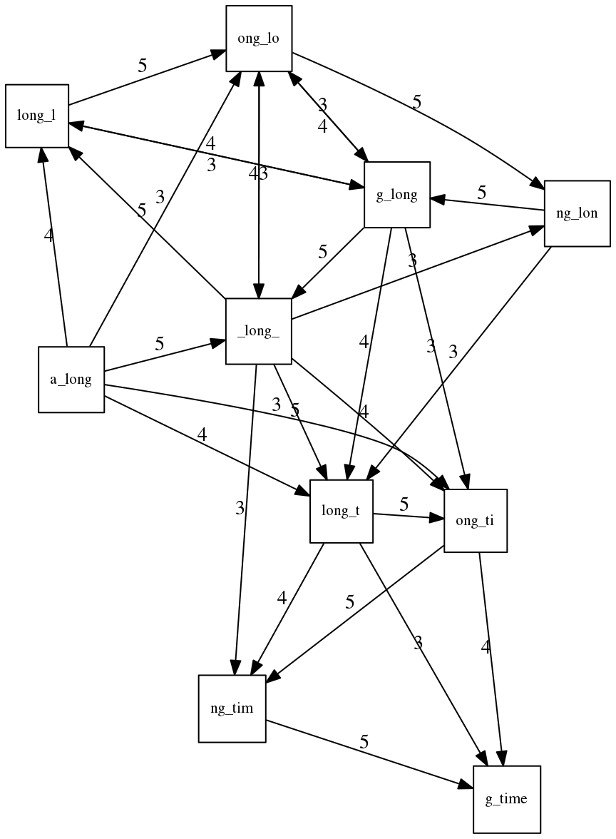 > <small>**An overlap graph** for with overlap length <code> >= 3<code>.</small> --- If we proceed with Greedy SCS we will follow the following trajectory through the graph: >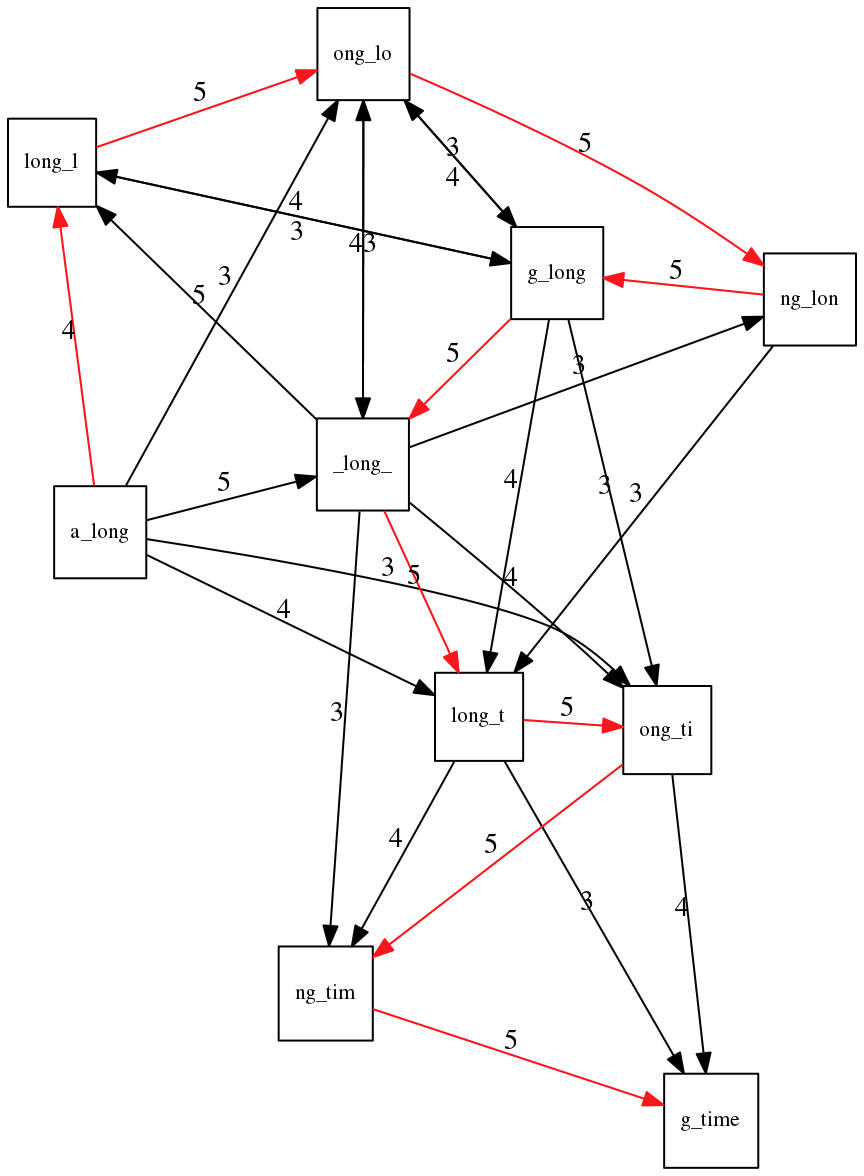 --- To make things even clearer let's isolate the path: 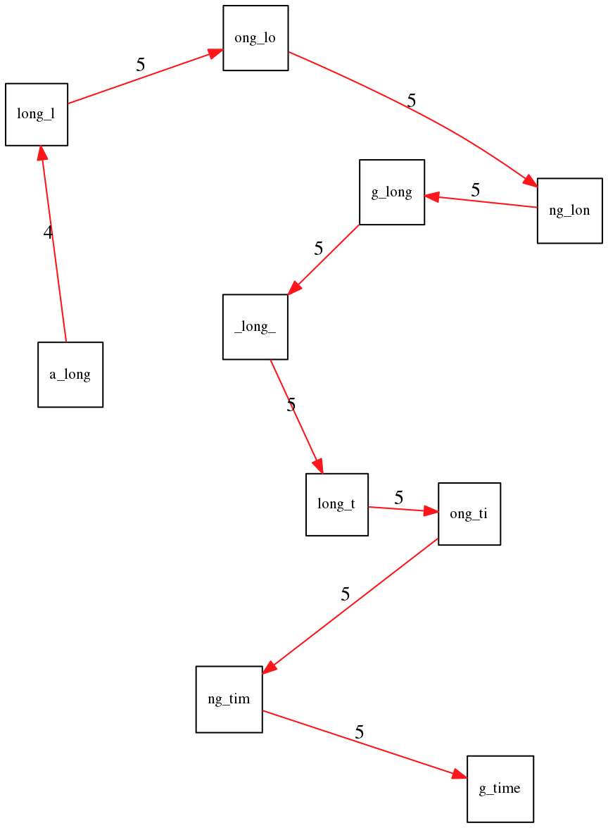 --- The total overlap here (the sum of edge weights) is 4+5+5+5+5+5+5+5+5=44 but it gives us `a_long_long_time` as the shortest superstring: ``` a_long long_l ong_lo ng_lon g_long _long_ long_t ong_ti ng_tim g_time ---------------- a_long_long_time ``` --- We are missing one instance of 'long' in this string. The following graph shows the path that would return the *correct* string: >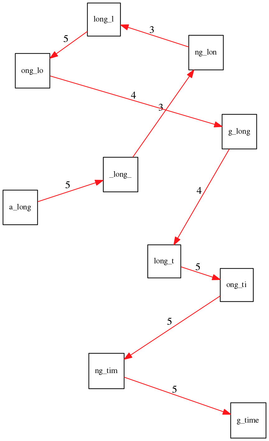 --- A path yielding the correct string with three repeats. The total overlap here is 5+3+3+5+4+4+5+5+5=39, which is *worse* than the previous path if our goal is to find the shortest superstring: ``` a_long _long_ ng_lon long_l ong_lo g_long long_t ong_ti ng_tim g_time --------------------- a_long_long_long_time ``` --- ## Are we really looking for the shortest superstring? As we've seen above the shortest common superstring (SCS) is: 1. **Difficult to obtain** as Greedy SCS algorithm does not guarantee finding it. So the answer we get may be longer than the real genome we are trying to assemble. 2. **May be shorter than we want** because if the genome contains repeats that are longer than the reads we are using, Greedy SCS will collapse them and make assembly shorter that the genome we are trying to get. Let's talk about an alternative way to represent the relationship between *k*-mers that may give us a more efficient algorithm. --- # de Bruijn graphs [Nicolaas de Bruijn](https://en.wikipedia.org/wiki/Nicolaas_Govert_de_Bruijn) had a purely theoretical interest of constructing _k_-universal strings for an arbitrary value of _k_. A _k_-universal string contains every possible _k_-mer only once: >[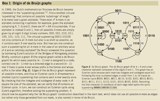](http://www.nature.com/nbt/journal/v29/n11/abs/nbt.2023.html) > >**de Bruijn graph**. From [Compeau:2011](http://www.nature.com/nbt/journal/v29/n11/abs/nbt.2023.html) --- This problem is equivalent to a string reconstruction problem we have been talking about above: finding a _k_-universal string is equivalent to finding a Hamiltonian path in an overlap graph constructed from all _k_-mers. Yet finding a Hamiltonian path in a really large graph (representing a real genome) is not a tractable problem as we have seen. Instead de Bruijn decided to represent _k_-mer composition in a graph using a slightly different logic. Again, suppose we have a "genome" <ode>TAATGCCATGGGATGTT</code> split in a collection of 3-mers: <samp> TAA AAT ATG TGC GCC CCA CAT ATG TGG GGG GGA GAT ATG TGT GTT </samp> --- We will assign 3-mers to _edges_ instead of _nodes_:  **_k_-mers as edges**. Edges represented by 3-mers connect nodes representing the overlaps. (Fig. 4.12 from [CP](http://bioinformaticsalgorithms.com/)) This graph can be simplified by gluing identical nodes together:  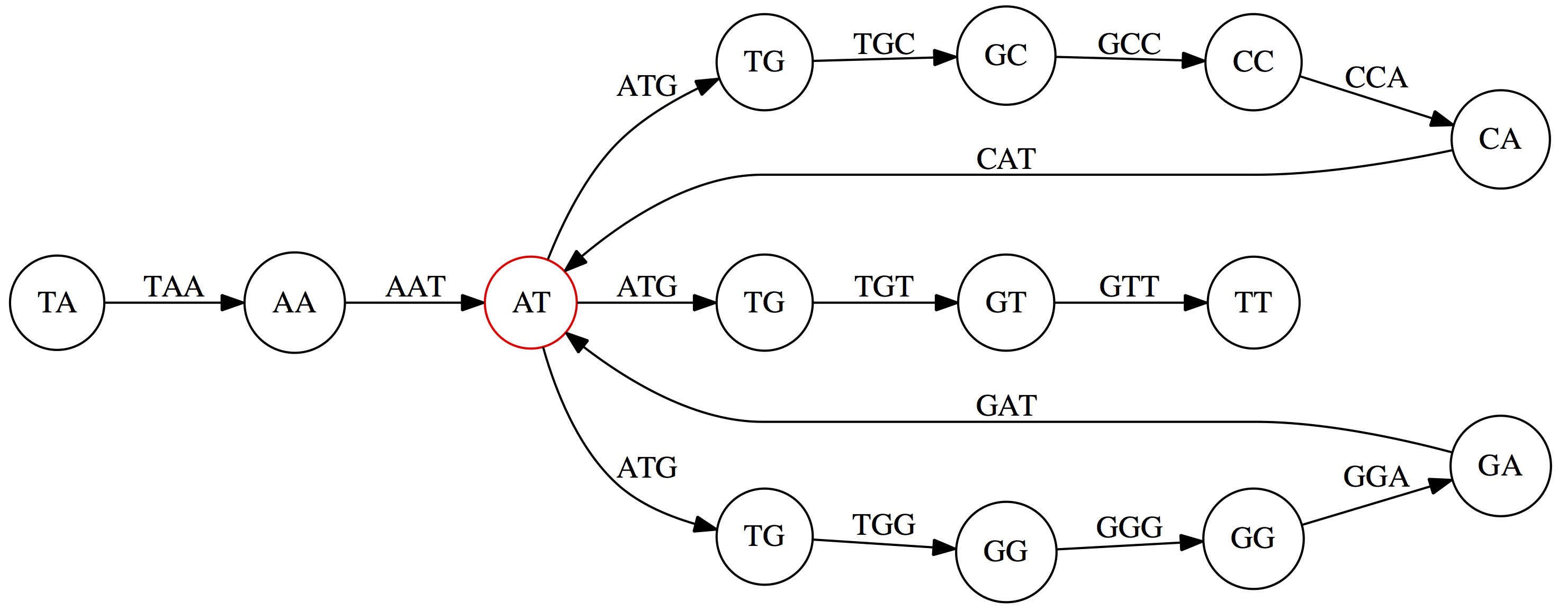 --- Here the complexity of the graph is reduced by first gluing redundant <font color="red">`AT`</font> nodes 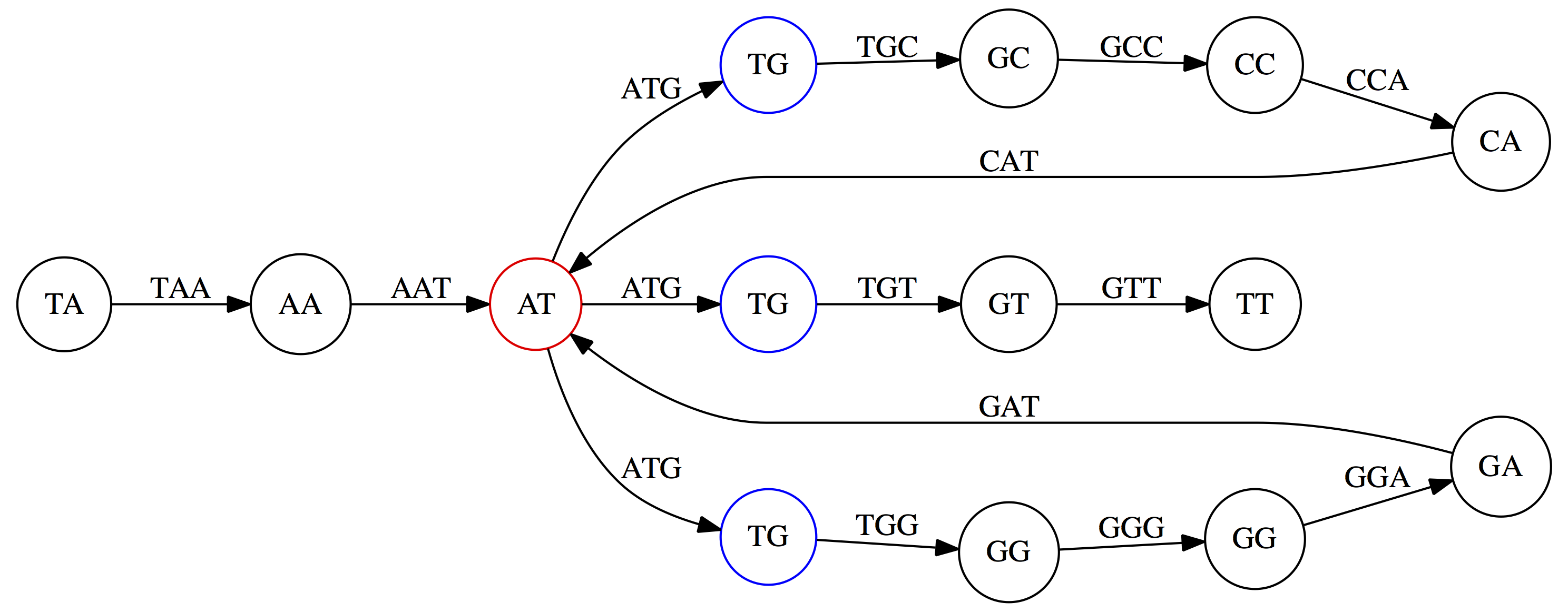 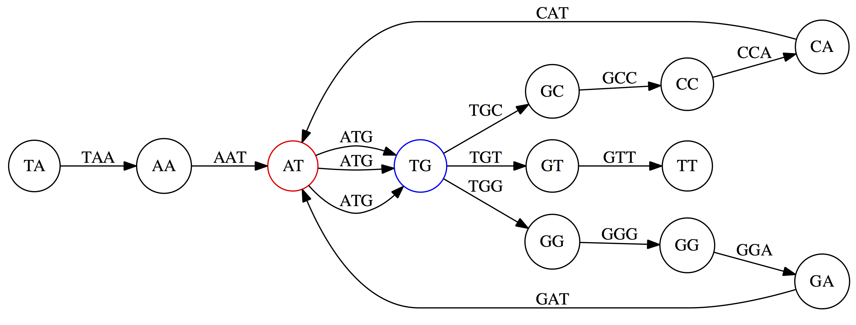 --- Next, <font color="blue">`TG`</font> nodes are merged 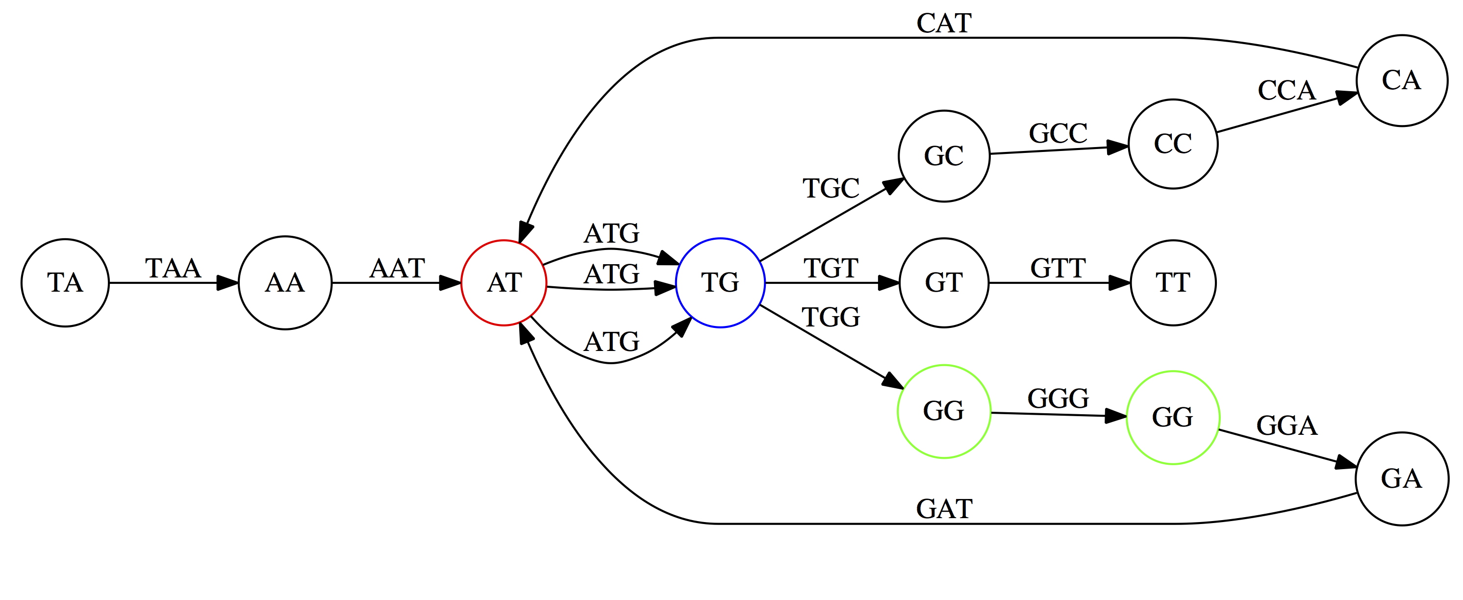 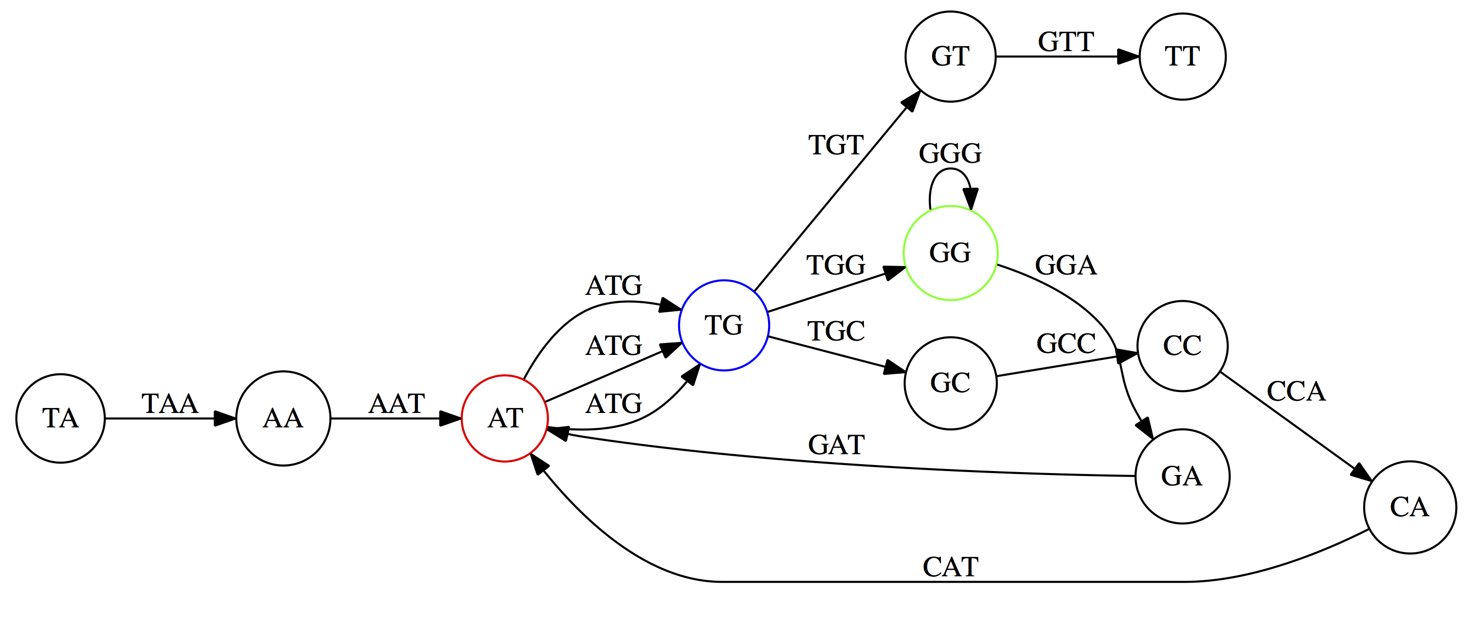 --- And, finally the two <font color="green">`GG`</font> nodes are resolved. (Fig. 4.13 from [CP](http://bioinformaticsalgorithms.com/)) Because we now represent _k_-mers as edges (rather than nodes), our problem has morphed into finding a path that visits every _edge_ once, or an [Eulerian Path](https://en.wikipedia.org/wiki/Eulerian_path): 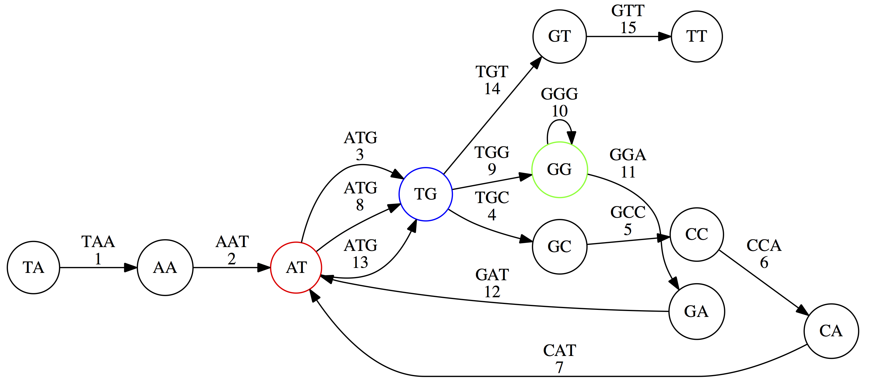 **Eulerian paths for the 15 3-mers**. Numbering of edges provides a way to reconstruct the original "genome". (Fig. 4.15 from [CP](http://bioinformaticsalgorithms.com/)) --- ## Euler's Theorem Some definitions: * **Balanced node** - a node where the number of incoming edges is equal to the number of outgoing edges * **Balanced graph** - a graph where all nodes are balanced * **Strongly connected graph** - any node can be reached from any other node **Euler's Theorem**: >Every balanced, strongly connected directed graph is Eulerian. --- Let's apply Euler's Theorem to a classical problem: The bridges of Königsberg problem. Here the question is: *Can you walk through all of Königsberg traversing every bridge exactly one time?* In other words: *Is there a Eulerian path through the city of Königsberg?* >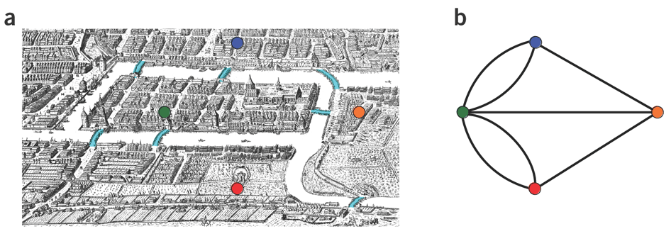 > >**Königsberg and Euler's Theorem**. (a) A map of old Königsberg, in which each area of the city is labeled with a different color point. (b) The Königsberg Bridge graph, formed by representing each of four land areas as a node and each of the city's seven bridges as an edge. (From [Campeau:2011](http://www.nature.com/nbt/journal/v29/n11/abs/nbt.2023.html#close)) By looking at this graph we can see that it is *unbalanced*. If one arrives to, say, the <font color="orange">orange</font> node from the <font color="blue">blue</font> node there are two ways to get out. Thus there is no way to see all of the city and traverse every bridge once! --- ## Repeats are still a challenge Let's look at the de Bruijn graph from above again. But this time let's drop edge numbering and pretend that the genome is now really known to us (as is usually the case in real life): >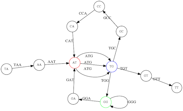 > >**Eulerian paths for the 15 3-mers**. --- In the original sequence `TAATGCCATGGGATGTT` *k*-mer <font color="red">`AT`</font> is present 3 times and *k*-mer <font color="blue">`TG`</font> is found twice. Thus *multiple* Eulerian walks are now possible like this: >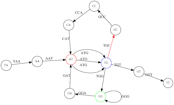 > >**Possible path #1**. Here after we reach <font color="blue">`TG`</font> node we turn **up**. --- The above path spells out: ``` TAA AAT ATG TGC GCC CCA CAT ATG TGG GGG GGA GAT ATG TGT GTT ----------------- TAATGCCATGGGATGTT ``` --- Yet there is an alternative: >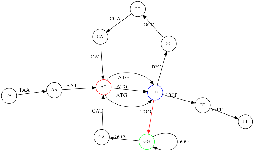 > >**Possible path #2**. Here after we reach <font color="blue">`TG`</font> node we turn **dow**. --- Which spells: ``` TAA AAT ATG TGG GGA GAT ATG TGC GCC CCA CAT ATG TGT GTT ---------------- TAATGGATGCCATGTT ``` Note how different these are: ``` TAATGCCATGGGATGTT TAATGGATGCCATGTTT ``` and only one of them is correct. Repeats are evil! --- ## *k*-mer size affects repeat resolution In the above example we have used *k*-mer size of 3. But what if we try 4 or 5? Below are De Bruijn graphs for different values of *k*: #### *k* = 3 >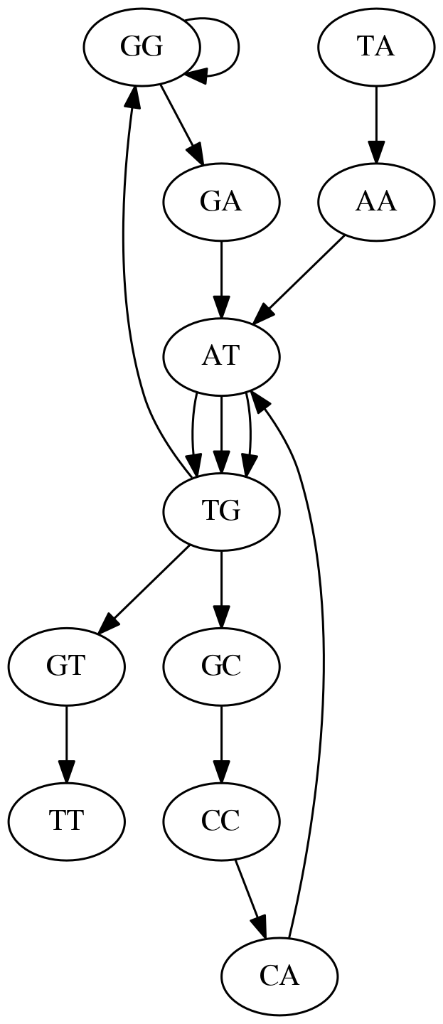 --- >This is our original graph #### *k* = 4 >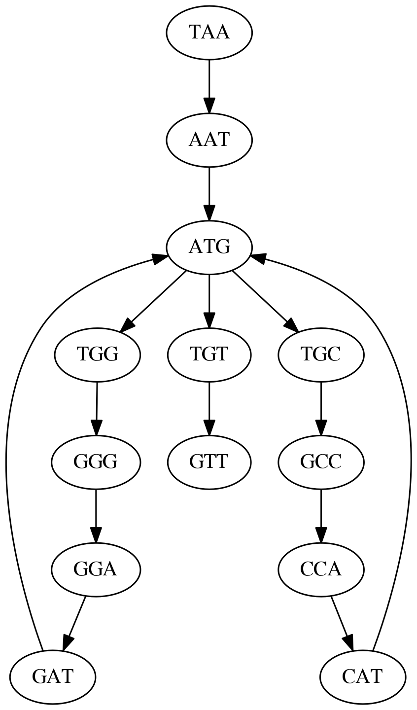 > >Here complexity is decreasing, but we still have the problem with having `ATG` twice. --- .pull-left[ #### *k* = 5 In this case there is only one path. This because our *k* is larger that the repeat size, so we can resolve it accurately. This is why technologies producing long sequencing reads stimulate so much enthusiasm - they will allow to resolve and produce accurate assembly of large genomes. ] .pull-right[  ] --- # Assembly in real life In this topic we've learned about two ways of representing the relationship between reads derived from a genome we are trying to assemble: 1. **Overlap graphs** - nodes are reads, edges are overlaps between reads. 2. **De Bruijn graphs** - nodes are overlaps, edges are reads. > --- **A**.  --- **B.** An overlap (A) and De Bruijn (B) graphs for the same string. Whatever the representation will be it will be messy: 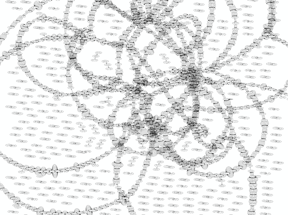 A fragment of a very large De Bruijn graph (Image from [BL](https://github.com/BenLangmead/ads1-slides/blob/master/0580_asm__practice.pdf)). --- There are multiple reasons for such messiness: **Sequence errors** Sequencing machines do not give perfect data. This results in spurious deviations on the graph. Some sequencing technologies such as Oxford Nanopore have very high error rate of ~15%. >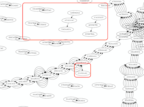 > >Graph components resulting from sequencing errors (Image from [BL](https://github.com/BenLangmead/ads1-slides/blob/master/0580_asm__practice.pdf)). --- **Ploidy** As we discussed earlier humans are diploid and there are multiple differences between maternal and paternal genomes. This creates "bubbles" on assembly graphs: >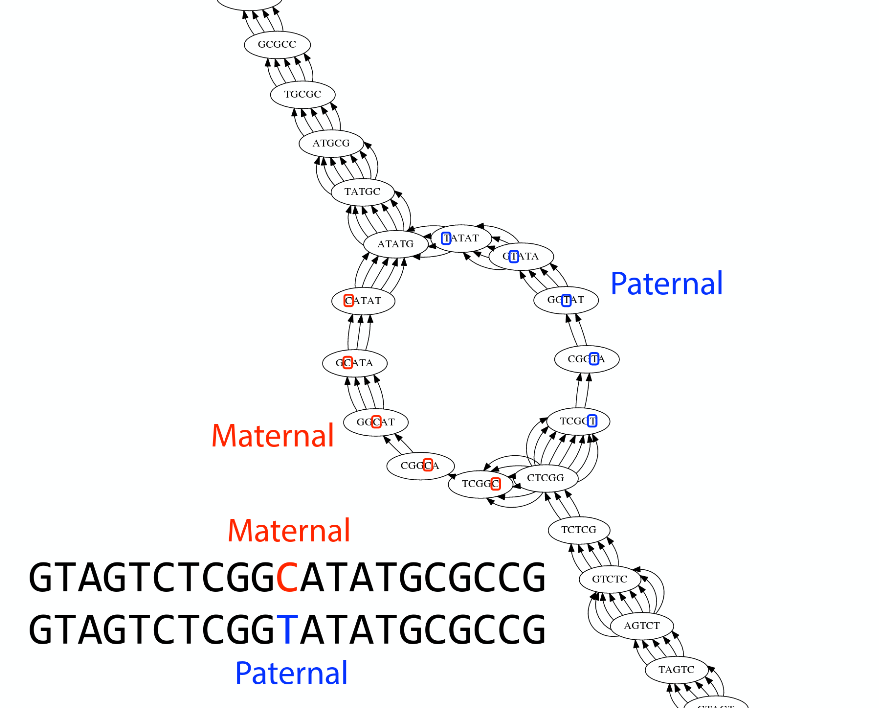 > >Bubbles due to a heterozygous site (Image from [BL](https://github.com/BenLangmead/ads1-slides/blob/master/0580_asm__practice.pdf)). --- **Repeats** As we've seen the third law of assembly is unbeatable. As a result some regions of the genome simply cannot be resolved and are reported in segments called *contigs*: >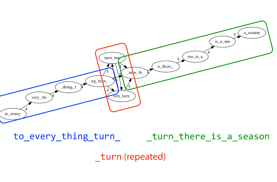 > >The following "genomic" segment will be reported in three pieces corresponding to regions flanking the repeat and repeat itself (Image from [BL](https://github.com/BenLangmead/ads1-slides/blob/master/0580_asm__practice.pdf)). --- .enlarge120[ # **How to perform Assembly with Galaxy?** ] --- See the tutorial accompanied by these slides! --- ### <i class="fas fa-key" aria-hidden="true"></i><span class="visually-hidden">keypoints</span> Key points - We learned about the strategies used by assemblers for hybrid assemblies - We performed an hybrid assembly of a bacterial genome and its annotation - Unicycler is a pipeline bases on Spades and Pilon dedicated to hybrid assembly of Small genomes - Combination of short and long reads helped us produce an almost perfect assembly --- ## Thank You! This material is the result of a collaborative work. Thanks to the [Galaxy Training Network](https://training.galaxyproject.org) and all the contributors! <div markdown="0"> <div class="contributors-line"> <table class="contributions"> <tr> <td><abbr title="These people wrote the bulk of the tutorial, they may have done the analysis, built the workflow, and wrote the text themselves.">Author(s)</abbr></td> <td> <a href="/training-material/hall-of-fame/nekrut/" class="contributor-badge contributor-nekrut"><img src="https://avatars.githubusercontent.com/nekrut?s=36" alt="Anton Nekrutenko avatar" width="36" class="avatar" /> Anton Nekrutenko</a><a href="/training-material/hall-of-fame/delphine-l/" class="contributor-badge contributor-delphine-l"><img src="/training-material/assets/images/orcid.png" alt="orcid logo" width="36" height="36"/><img src="https://avatars.githubusercontent.com/delphine-l?s=36" alt="Delphine Lariviere avatar" width="36" class="avatar" /> Delphine Lariviere</a><a href="/training-material/hall-of-fame/slugger70/" class="contributor-badge contributor-slugger70"><img src="/training-material/assets/images/orcid.png" alt="orcid logo" width="36" height="36"/><img src="https://avatars.githubusercontent.com/slugger70?s=36" alt="Simon Gladman avatar" width="36" class="avatar" /> Simon Gladman</a> </td> </tr> <tr class="reviewers"> <td><abbr title="These people reviewed this material for accuracy and correctness">Reviewers</abbr></td> <td> <a href="/training-material/hall-of-fame/shiltemann/" class="contributor-badge contributor-badge-small contributor-shiltemann"><img src="https://avatars.githubusercontent.com/shiltemann?s=36" alt="Saskia Hiltemann avatar" width="36" class="avatar" /></a><a href="/training-material/hall-of-fame/nsoranzo/" class="contributor-badge contributor-badge-small contributor-nsoranzo"><img src="https://avatars.githubusercontent.com/nsoranzo?s=36" alt="Nicola Soranzo avatar" width="36" class="avatar" /></a><a href="/training-material/hall-of-fame/hexylena/" class="contributor-badge contributor-badge-small contributor-hexylena"><img src="https://avatars.githubusercontent.com/hexylena?s=36" alt="Helena Rasche avatar" width="36" class="avatar" /></a><a href="/training-material/hall-of-fame/gallardoalba/" class="contributor-badge contributor-badge-small contributor-gallardoalba"><img src="https://avatars.githubusercontent.com/gallardoalba?s=36" alt="Cristóbal Gallardo avatar" width="36" class="avatar" /></a><a href="/training-material/hall-of-fame/willdurand/" class="contributor-badge contributor-badge-small contributor-willdurand"><img src="https://avatars.githubusercontent.com/willdurand?s=36" alt="William Durand avatar" width="36" class="avatar" /></a><a href="/training-material/hall-of-fame/nekrut/" class="contributor-badge contributor-badge-small contributor-nekrut"><img src="https://avatars.githubusercontent.com/nekrut?s=36" alt="Anton Nekrutenko avatar" width="36" class="avatar" /></a><a href="/training-material/hall-of-fame/bgruening/" class="contributor-badge contributor-badge-small contributor-bgruening"><img src="https://avatars.githubusercontent.com/bgruening?s=36" alt="Björn Grüning avatar" width="36" class="avatar" /></a><a href="/training-material/hall-of-fame/bebatut/" class="contributor-badge contributor-badge-small contributor-bebatut"><img src="https://avatars.githubusercontent.com/bebatut?s=36" alt="Bérénice Batut avatar" width="36" class="avatar" /></a><a href="/training-material/hall-of-fame/delphine-l/" class="contributor-badge contributor-badge-small contributor-delphine-l"><img src="https://avatars.githubusercontent.com/delphine-l?s=36" alt="Delphine Lariviere avatar" width="36" class="avatar" /></a><a href="/training-material/hall-of-fame/njall/" class="contributor-badge contributor-badge-small contributor-njall"><img src="https://avatars.githubusercontent.com/njall?s=36" alt="Niall Beard avatar" width="36" class="avatar" /></a></td> </tr> </table> </div> </div> <div style="display: flex;flex-direction: row;align-items: center;justify-content: center;"> <img src="/training-material/assets/images/GTNLogo1000.png" alt="Galaxy Training Network" style="height: 100px;"/> </div> Tutorial Content is licensed under <a rel="license" href="http://creativecommons.org/licenses/by/4.0/">Creative Commons Attribution 4.0 International License</a>.<br/>