Why is it important to perform quality control and remove contamination from raw metagenomic reads before assembly?
What is the purpose of binning in metagenomic analysis? How does binning help in reconstructing metagenome-assembled genomes (MAGs) from complex microbial communities?
What metrics are commonly used to assess the quality of MAGs? How do completeness and contamination levels affect the reliability of downstream analyses?
How does taxonomic assignment contribute to the analysis of MAGs? What databases or tools can be used for assigning taxonomy, and why is it important to use up-to-date references?
What is the significance of functional annotation in metagenomic studies? How can tools like Bakta help uncover the biological roles of microbial communities?
Objectives:
List the key steps involved in MAGs building from raw data.
Define essential terms such as MAGs (Metagenome-Assembled Genomes), binning, and functional annotation.
Explain the importance of preprocessing metagenomic reads, including quality control and contamination removal.
Describe the purpose and process of assembling, binning, and refining MAGs.
Compare the quality of MAGs based on completeness, contamination, and other metrics.
Assess the quality of MAGs and determine whether they meet standards for downstream analysis.
Summarize how taxonomic assignment and functional annotation contribute to understanding microbial communities.
Evaluate the reliability of taxonomic assignments and functional annotations based on reference databases.
Analyze the relative abundance of microbial taxa in the samples and infer ecological dynamics.
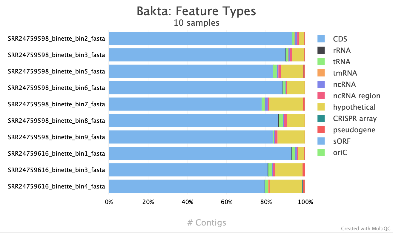
Identify the types of genomic features annotated by Bakta (e.g., CDS, rRNA, tRNA).
Interpret the functional annotation results to identify metabolic pathways, virulence factors, and other biological roles.
Metagenomics has revolutionized our understanding of microbial communities by enabling the study of genetic material directly from environmental samples. One of the most powerful applications of metagenomics is the reconstruction of Metagenome-Assembled Genomes (MAGs), i.e. near-complete or complete genomes of individual microorganisms recovered from complex microbial communities. MAGs provide invaluable insights into microbial diversity, function, and ecology, without the need for laboratory cultivation.
This tutorial is designed for anyone interested in reconstructing MAGs from paired short metagenomic reads. You will learn the essential steps, from quality control and read preprocessing to assembly, binning, refinement, and annotations of MAGs. By the end of this tutorial, you will be equipped with the knowledge, tools, and workflows to confidently generate high-quality MAGs from your own metagenomic datasets.
To illustrate the workflows, we will use public data from a study investigating the response of the honey bee gut microbiota to Nosema ceranae (a highly prevalent microsporidian parasite) under the influence of a probiotic and/or a neonicotinoid insecticide (Sbaghdi et al. 2024). The honey bee gut microbiome comprises a relatively simple core community dominated by five bacterial lineages, including Snodgrassella alvi and Gilliamella apicola, which play essential roles in digestion, immunity, and pathogen defense (Motta and Moran 2024). However, this microbiome is highly sensitive to abiotic stressors, such as pesticides, pollutants, and climate change (Motta and Moran 2024, Ramsey et al. 2019, Alberoni et al. 2021). For example, exposure to neonicotinoids has been linked to shifts in microbial diversity and increased susceptibility to opportunistic pathogens Alberoni et al. 2021.
While research often examines stressors in isolation, their synergistic effects remain understudied (Paris et al. 2020, Meixner and others 2010). In the Sbaghdi et al. 2024 study, western honey bees were experimentally infected with N. ceranae spores, exposed to the neonicotinoid thiamethoxam, and/or treated with the probiotic bacterium Pediococcus acidilactici, which is thought to enhance tolerance to N. ceranae. The study used deep shotgun metagenomic Illumina sequencing to analyze 21 samples, with taxonomic composition explored using MetaPhlAn4 (Blanco-Mı́guez Aitor et al. 2023).
A well-organized workspace is essential for efficient and reproducible metagenomic analysis. In Galaxy, each analysis should be conducted within its own dedicated history to ensure clarity, avoid data mixing, and streamline collaboration or future reference.
Hands On: Prepare history
Create a new history for this analysis
To create a new history simply click the new-history icon at the top of the history panel:
Rename the history
Click on galaxy-pencil (Edit) next to the history name (which by default is “Unnamed history”)
Type the new name
Click on Save
To cancel renaming, click the galaxy-undo “Cancel” button
If you do not have the galaxy-pencil (Edit) next to the history name (which can be the case if you are using an older version of Galaxy) do the following:
Click on Unnamed history (or the current name of the history) (Click to rename history) at the top of your history panel
Type the new name
Press Enter
To proceed with our analysis, we need to import the raw metagenomic sequencing data from the NCBI Sequence Read Archive (SRA). For this tutorial, we use two representative datasets, identified by their SRA run accession numbers: SRR24759598 and SRR24759616. These datasets will serve as the starting point for our quality control, preprocessing, and MAG reconstruction workflows. Let’s retrieve and prepare these reads for downstream analysis.
Hands On: Get data from NCBI SRA
Create a new file with one SRA per line
SRR24759598
SRR24759616
Click galaxy-uploadUpload Data at the top of the tool panel
Select galaxy-wf-editPaste/Fetch Data at the bottom
Paste the file contents into the text field
Press Start and Close the window
Faster Download and Extract Reads in FASTQ ( Galaxy version 3.1.1+galaxy1)
“select input type”: List of SRA accession, one per line
param-file“sra accession list”: created dataset
Rename Pair-end data (fasterq-dump) collection to Raw reads
Comment
Download from NCBI SRA can take time. If it takes too long, you can import the data from Zenodo.
Hands On: Import raw data
Import the two files from ENA or the Shared Data library:
Create a collection named Raw reads, rename the pairs with the sample name (SRR24759598 and SRR24759616)
Preprocess the Reads
The quality and composition of our metagenomic dataset directly influence the success of Metagenome-Assembled Genome (MAG) reconstruction. To ensure accurate, high-resolution results, it is essential to preprocess the reads through a series of critical steps:
Quality Control: Assess and refine sequencing data to remove low-quality bases, adapters, and short reads that could compromise downstream analyses.
Contamination Removal: Filter out host-derived sequences (e.g., honey bee DNA) and potential human contaminants, which can obscure microbial signals and introduce bias.
By meticulously preparing the reads, we create a clean, microbial-enriched dataset—the optimal foundation for robust MAG reconstruction. Let’s walk through these essential preprocessing steps.
Control Raw Data Quality
Poor-quality reads, such as those with low base-calling accuracy, adapter contamination, or insufficient length, can introduce errors, bias assemblies, and compromise the integrity of your results. Before proceeding with any analysis, it is essential to assess, trim, and filter our raw sequencing data to ensure only high-quality reads are retained.
Trim and filter reads using fastp (Chen et al. 2018), removing low-quality bases (default: minimum quality score of 15) and short reads (default: minimum length of 15 bases). These parameters can be adjusted based on your specific dataset and requirements.
Aggregate quality reports for all samples into a single, comprehensive overview using MultiQC (Ewels et al. 2016), allowing to quickly visualize and compare the quality metrics across the datasets.
Comment
Learn more about sequencing data quality control in our dedicated tutorial: Quality Control
Let’s import the workflow from WorkflowHub:
Hands On: Importing and Launching a WorkflowHub.eu Workflow
Click on galaxy-workflows-activityWorkflows in the Galaxy activity bar (on the left side of the screen, or in the top menu bar of older Galaxy instances). You will see a list of all your workflows
Click on galaxy-uploadImport at the top-right of the screen
On the new page, select the GA4GH servers tab, and configure the GA4GH Tool Registry Server (TRS) Workflow Search interface as follows:
Select the version you would like to galaxy-upload import
The workflow will be imported to your list of workflows. Note that it will also carry a little blue-white shield icon next to its name, which indicates that this is an original workflow version imported from a TRS server. If you ever modify the workflow with Galaxy’s workflow editor, it will lose this indicator.
Below is a short video showing the entire uncomplicated procedure:
Video: Importing via search from WorkflowHub
We can now launch it:
Hands On: Control raw data quality
Run the workflow using the following parameters
param-collection“Raw reads”: Raw reads collection
“Qualified quality score”: 15
“Minimal read length”: 15
Inspect the MultiQC report
Question
How many reads are in each dataset?
What are the length of the reads before trimming?
What are the miminum values for average bp quality score for forward and reverse reads, before and and after trimming and filtering?
43.9 millions reads for SRR24759598 and 42.8 millions for SRR24759616
150 bp
Minimum average bp quality scores given the “Sequence Quality” graph:
SRR24759598
SRR24759616
Forward (Read 1) - Before
34.5
34.6
Forward (Read 1) - After
34.5
34.6
Reverse (Read 2) - Before
33.4
32.7
Reverse (Read 2) - After
33.4
32.7
Remove Contamination and Host Reads
Metagenomic datasets often contain non-microbial sequences that can compromise the accuracy and quality of downstream analyses, including MAG reconstruction. These sequences may originate from host DNA (in this case, the honey bee) or external contamination, such as human DNA introduced during sample handling or sequencing. Failing to remove these sequences can lead to misassembly, incorrect taxonomic assignments, and skewed functional interpretations.
We will now focus on filtering out both host (bee) and potential human contamination from our metagenomic reads. This critical step ensures that our dataset is enriched for microbial sequences, improving the reliability of our MAGs and enabling more precise biological insights. We will use a dedicated workflow to:
Map reads against reference genomes for the host (bee) and common contaminants using Bowtie2 (Langmead et al. 2009, Langmead and Salzberg 2012), enabling precise identification and removal of non-microbial sequences.
Aggregate and visualize mapping results with MultiQC (Ewels et al. 2016), providing a comprehensive overview of the filtering process and ensuring transparency in our data cleaning efforts.
Let’s import the workflow from WorkflowHub:
Hands On: Importing and Launching a WorkflowHub.eu Workflow
Launch host-contamination-removal-short-reads/main (v1) (View on WorkflowHub)
Click on galaxy-workflows-activityWorkflows in the Galaxy activity bar (on the left side of the screen, or in the top menu bar of older Galaxy instances). You will see a list of all your workflows
Click on galaxy-uploadImport at the top-right of the screen
On the new page, select the GA4GH servers tab, and configure the GA4GH Tool Registry Server (TRS) Workflow Search interface as follows:
Select the version you would like to galaxy-upload import
The workflow will be imported to your list of workflows. Note that it will also carry a little blue-white shield icon next to its name, which indicates that this is an original workflow version imported from a TRS server. If you ever modify the workflow with Galaxy’s workflow editor, it will lose this indicator.
Below is a short video showing the entire uncomplicated procedure:
Video: Importing via search from WorkflowHub
We will run the workflow twice:
First, we focus on filtering out host (honey bee) reads, i.e. sequences originating from the bee itself, which can dominate the dataset and obscure microbial signals
Second, we will target potential human contamination, which may have been introduced during sample handling or sequencing.
Let’s begin by launching the workflow to remove honey bee-derived sequences.
“Host/Contaminant Reference Genome”: A. mellifera genome (apiMel3, Baylor HGSC Amel_3.0)
Click on Workflows on the Activity Bar on the left.
At the top of the resulting page you will have the option to switch between the My workflows, Workflows shared with me and Public workflows tabs.
Select the tab you want to see all workflows in that category
Search for your desired workflow.
Click on the workflow name: a pop-up window opens with a preview of the workflow.
To run it directly: click Run (top-right).
Recommended: click Import (left of Run) to make your own local copy under Workflows / My Workflows.
Rename Reads without host or contaminant reads collection to Reads without bee reads
Inspect the MultiQC report
Question
Which percentage of reads mapped to the honey bee reference genome?
How many reads have been removed?
2.8% for SRR24759598 and 1.1% for SRR24759616
2.8% for SRR24759598 and 1.1% for SRR24759616
With the host (honey bee) sequences successfully filtered out, we now turn our attention to removing potential human contamination from the dataset. We run the workflow a second time, this time aligning the reads against a human reference genome:
Hands On: Remove human reads
Run the workflow using the following parameters
param-collection“Short-reads”: Reads without bee reads collection
“Host/Contaminant Reference Genome”: Human (Homo sapiens): hg38 Full
Rename Reads without host or contaminant reads collection to Reads without bee and human reads
Inspect the newly generated MultiQC report
Question
Which percentage of reads mapped to the honey bee reference genome?
How many reads have been removed?
0.1% in both samples
We have now completed the essential preprocessing steps to ensure our metagenomic dataset is clean, high-quality, and enriched for microbial sequences. By performing rigorous quality control and systematically removing host and contaminant reads, we have minimized potential biases and maximized the reliability of our data. With these preparations complete, our dataset is now optimized for the next phase: assembling and reconstructing Metagenome-Assembled Genomes (MAGs).
Build, Refine, and Annotate Metagenome-Assembled Genomes (MAGs)
Now that our metagenomic reads are clean, high-quality, and free of contamination, we are ready to embark on the core phase of our analysis: reconstructing and annotating Metagenome-Assembled Genomes (MAGs). This process transforms our processed sequencing data into near-complete or complete microbial genomes, enabling deeper insights into the functional potential, taxonomy, and ecological roles of the microorganisms in our samples.
We will use a comprehensive workflow to go through each step of MAG reconstruction and annotation:
Assembly: Reconstruct genomic sequences (contigs) from our metagenomic reads using MEGAHIT (Li et al. 2015) or metaSPADES (Nurk et al. 2017).
Binning: Group contigs into discrete genomic bins using four complementary tools: MetaBAT2 (Kang et al. 2019), MaxBin2 (Wu et al. 2015), SemiBin (Pan et al. 2022), and CONCOCT (Alneberg et al. 2014), each offering unique strengths for capturing microbial diversity.
Refinement: Improve the quality and completeness of the MAGs by refining bins with Binette (Mainguy and Hoede 2024), the successor to metaWRAP, which removes contamination and merges related bins.
Dereplication: Consolidate the MAGs across all input samples using dRep (Olm et al. 2017), which clusters genomes based on CheckM2 quality metrics to eliminate redundancy.
Quality Assessment: Evaluate the integrity of the MAGs with CheckM (Parks et al. 2015) and CheckM2 (Chklovski et al. 2023) for completeness and contamination estimates.
Abundance Estimation: Quantify the relative abundance of each MAG in our samples using CoverM (Aroney et al. 2025), providing insights into microbial population dynamics.
Taxonomic Assignment: Classify the MAGs using GTDB-Tk (Chaumeil et al. 2019), aligning them with the Genome Taxonomy Database for accurate taxonomic placement.
Functional Annotation: Identify and annotate genes within our MAGs using Bakta (Schwengers et al. 2021), revealing their functional potential and biological roles.
All results are consolidated into a single MultiQC (Ewels et al. 2016) report, allowing us to easily visualize and interpret the quality and characteristics of our MAGs.
Let’s import the workflow from WorkflowHub:
Hands On: Importing and Launching a WorkflowHub.eu Workflow
Click on galaxy-workflows-activityWorkflows in the Galaxy activity bar (on the left side of the screen, or in the top menu bar of older Galaxy instances). You will see a list of all your workflows
Click on galaxy-uploadImport at the top-right of the screen
On the new page, select the GA4GH servers tab, and configure the GA4GH Tool Registry Server (TRS) Workflow Search interface as follows:
“TRS Server”: workflowhub.eu
“search query”: name:"mags-building/main"
Expand the correct workflow by clicking on it
Select the version you would like to galaxy-upload import
The workflow will be imported to your list of workflows. Note that it will also carry a little blue-white shield icon next to its name, which indicates that this is an original workflow version imported from a TRS server. If you ever modify the workflow with Galaxy’s workflow editor, it will lose this indicator.
Below is a short video showing the entire uncomplicated procedure:
Video: Importing via search from WorkflowHub
Hands On: Build, refine, and annotate MAGs
Run the workflow using the following parameters
“Trimmed reads from grouped samples”: Reads without bee and human reads
“Trimmed reads”: Reads without bee and human reads
“Choose Assembler”: MEGAHIT
Comment
metaSPAdes is an alternative assembler.
MEGAHIT is less computationally intensive and generate higher quality single and shorter contigs but shorter. metaSPAdes is very computationally intensive, but generates longer/more complete assemblies.
“Minimum length of contigs to output”: 200
“Environment for the built-in model (SemiBin)”: global
Comment
Environment for the built-in model (SemiBin), options are:
human_gut,
dog_gut,
ocean,
soil,
cat_gut,
human_oral,
mouse_gut,
pig_gut,
built_environment,
wastewater,
chicken_caecum,
global
“Minimum MAG completeness percentage”: 75
Choosing a minimum genome completeness threshold is a critical but complex decision in de-replication and bin refinement. There is a trade-off between computational efficiency and genome quality:
Lower completeness thresholds allow more genomes to be included but reduce the accuracy of similarity comparisons.
Higher completeness thresholds improve accuracy but may exclude valuable genomes.
Impact of Genome Completeness on Aligned Fractions
When genomes are incomplete, the aligned fraction—the proportion of the genome that can be compared—decreases. For example, if you randomly sample 20% of a genome twice, the aligned fraction between these subsets will be low, even if they originate from the same genome.
This effect is illustrated below, where lower completeness thresholds result in a wider range of aligned fractions, reducing the reliability of similarity metrics like ANI.
Effect on Mash ANI
Incomplete genomes also artificially lower Mash ANI values, even for identical genomes. As completeness decreases, the reported Mash ANI drops, even when comparing identical genomes.
This is problematic because Mash is used for primary clustering in tools like dRep. If identical genomes are split into different primary clusters due to low Mash ANI, they will never be compared by the secondary algorithm and thus won’t be de-replicated.
Practical Implications for De-Replication
Primary Clustering Thresholds:
If you set a minimum completeness of 50%, identical genomes subset to 50% may only achieve a Mash ANI of \( \approx \) 96%. To ensure these genomes are grouped in the same primary cluster, the primary clustering threshold must be \( \leq \) 96%. Otherwise, they may be incorrectly separated.
Computational Trade-Offs:
Lower primary thresholds increase the size of primary clusters, leading to more secondary comparisons and longer runtimes. Higher thresholds improve speed but risk missing true matches.
Unknown Completeness:
In practice, the true completeness of genomes is often unknown. Tools like CheckM estimate completeness using single-copy gene inventories, but these estimates are not perfect in particular for phages and plasmids, explaining why they are not supported in dRep. In general though, checkM is pretty good at accessing genome completeness:
Guidelines for Setting Completeness Thresholds
Avoid thresholds below 50% completeness: Genomes below this threshold are often too fragmented for reliable comparisons, and secondary algorithms may fail.
Adjust Mash ANI thresholds accordingly: If you lower the secondary ANI threshold, also lower the Mash ANI threshold to ensure incomplete but similar genomes are grouped together.
Balancing genome completeness and computational efficiency is key to effective de-replication. While lower completeness thresholds include more genomes, they reduce alignment accuracy and increase runtime. Aim for a minimum completeness of \( \geq \)50% and adjust clustering thresholds to avoid splitting identical genomes.
“Contamination weight (Binette)”: 2
Comment
This weight is used for the scoring the bins. A low weight favor complete bins over low contaminated bins.
“Read length (CONCOCT)”: 150
Comment
CONCOCT requires the read length for coverage. Best use fastQC to estimate the mean value
“CheckM2 Database”: most recent one
Comment
This database is used for quality assessment for Binette, dRep, and quality assessment of the final bins.
“Minimum MAG length”: 50000
In dRep, the set of Metagenome-Assembled Genomes (MAGs) undergoes quality filtering before any comparisons are performed. This critical step ensures that only high-quality genomes are retained for downstream analysis, improving both accuracy and computational efficiency.
One of the first steps in quality filtering is length-based filtering. Genomes that do not meet the minimum length threshold are filtered out upfront. This avoids unnecessary CheckM computations and ensures that only sufficiently large genomes are processed.
Important Note: All genomes must contain at least one predicted Open Reading Frame (ORF). Without an ORF, CheckM may stall during processing. To prevent this, a minimum genome length of 10,000 base pairs (bp) is recommended.
The default minimum length threshold in dRep is 50,000 bp. This threshold strikes a balance between computational efficiency and genome quality, ensuring that only meaningful and sufficiently complete genomes are included in the de-replication process.
“ANI threshold for dereplication”: 0.95
Average Nucleotide Identity (ANI) is a computational metric used to quantify the genomic similarity between two microbial genomes. It measures the mean sequence identity across all orthologous regions—regions of the genome that are shared and aligned between the two organisms. ANI is widely used in microbial genomics and metagenomics to:
Compare the similarity of bacterial or archaeal genomes.
Define species boundaries (e.g., a threshold of 95–96% ANI is commonly used to delineate bacterial species).
Identify redundant genomes in datasets, such as Metagenome-Assembled Genomes (MAGs), for de-replication.
How ANI Is Calculated
Genome Alignment: The genomes of two organisms are compared using whole-genome alignment tools (e.g., BLAST, MUMmer, or FastANI). These tools identify regions of the genomes that are homologous (shared due to common ancestry).
Identity Calculation: For each aligned region, the percentage of identical nucleotides is calculated. ANI is then computed as the mean identity across all aligned regions that meet a specified length threshold (e.g., regions \( \geq \) 1,000 base pairs).
Normalization: ANI accounts for unaligned regions (e.g., due to genomic rearrangements or horizontal gene transfer) by focusing only on the aligned portions of the genomes. This ensures the metric reflects conserved genomic similarity rather than absolute sequence coverage.
Interpreting ANI Values ANI values range from 0% to 100%, where:
ANI \( \approx \) 100%: The genomes are nearly identical, likely representing strains of the same species or clones.
ANI \( \geq \) 95–96%: The genomes likely belong to the same species (a widely accepted threshold for bacterial species delineation).
ANI \( \approx \) 80–95%: The genomes belong to closely related species within the same genus.
ANI \( < \) 80%: The genomes are distantly related and likely belong to different genera or higher taxonomic ranks.
Applications of ANI
Species Delineation: ANI is a gold standard for defining microbial species, replacing or complementing traditional methods like DNA-DNA hybridization (DDH). For example, an ANI \(\geq \) 95% is often used to confirm that two genomes belong to the same species.
De-Replication of MAGs: In metagenomics, ANI is used to identify and remove redundant MAGs from datasets. MAGs with ANI values above a threshold (e.g., 99%) are considered redundant, and only the highest-quality representative is retained for downstream analysis.
Strain-Level Comparisons: ANI can distinguish between closely related strains of the same species, helping researchers study microbial diversity at fine taxonomic resolutions.
Taxonomic Classification: ANI is used to assign unknown genomes to known taxonomic groups by comparing them to reference genomes in databases.
Tools for Calculating ANI
Several bioinformatics tools are available to compute ANI, including:
FastANI ( Galaxy version 1.3) (Jain et al. 2018): A fast, alignment-free tool for estimating ANI between genomes.
PyANI: A Python-based tool that supports multiple ANI calculation methods (e.g., BLAST, MUMmer).
Limitations of ANI
While ANI is a powerful metric, it has some limitations:
Dependence on Alignment: ANI requires sufficiently aligned regions to be accurate. Highly divergent or rearranged genomes may yield unreliable ANI values.
Threshold Variability: The ANI threshold for species delineation (e.g., 95%) may vary depending on the microbial group or study context.
Computational Requirements: Calculating ANI for large datasets (e.g., thousands of MAGs) can be computationally intensive.
Average Nucleotide Identity (ANI) is a fundamental metric in microbial genomics, providing a robust way to compare genomes, define species, and refine metagenomic datasets. By leveraging ANI, researchers can ensure the accuracy and reliability of their genomic analyses, from species classification to de-replication of MAGs.
Selecting an appropriate ANI threshold for de-replication depends on the specific goals of your analysis. ANI measures the similarity between genomes, but the threshold for considering genomes “the same” varies by application. Two key parameters influence this decision:
Minimum secondary ANI: The lowest ANI value at which genomes are considered identical.
Minimum aligned fraction: The minimum genome overlap required to trust the ANI calculation.
These parameters are determined by the secondary clustering algorithm used in tools like dRep ( Galaxy version 3.6.2+galaxy1)
Common Use Cases and Thresholds
Species-Level De-Replication
For generating Species-Level Representative Genomes (SRGs), a 95% ANI threshold is widely accepted. This threshold was used in studies like Almeida et al. 2019 to create a comprehensive set of high-quality reference genomes for human gut microbes. While there is debate about whether bacterial species exist as discrete units or a continuum, 95% ANI remains a practical standard for species-level comparisons. For context, see Olm et al. 2017.
Avoiding Read Mis-Mapping
If the goal is to prevent mis-mapping of short metagenomic reads (typically (( \sim )) 150 bp), a stricter 98% ANI threshold is recommended. At this level, reads are less likely to map equally well to multiple genomes, ensuring clearer distinctions between closely related strains.
Default and Practical Considerations
Default ANI threshold in dRep:95% (suitable for most species-level applications).
Upper limit for detection: Thresholds up to 99.9% are generally reliable, but higher values (e.g., 100%) are impractical due to algorithmic limitations (e.g., genomic repeats). Self-comparisons typically yield (( \sim )) 99.99% ANI due to these constraints.
For strain-level comparisons, consider using InStrain ( Galaxy version 1.5.3+galaxy0) (Olm et al. 2021), which provides detailed strain-resolution analyses.
Important Notes
De-replication collapses closely related but non-identical strains/genomes. This is inherent to the process.
To explore strain-level diversity after de-replication, map original reads back to the dereplicated genomes and visualize the strain cloud using tools like InStrain (Bendall et al. 2016).
Contamination in Metagenome-Assembled Genomes (MAGs) refers to the presence of sequences from organisms other than the target organism. During de-replication, setting a maximum contamination threshold ensures that only high-quality, representative genomes are retained for downstream analyses.
Why Set a Maximum Contamination Threshold?
Data Quality:
High contamination can distort taxonomic classification, functional annotation, and comparative genomics. A contamination threshold ensures that only high-purity MAGs are included.
Accurate De-Replication:
Contaminated MAGs may cluster incorrectly, leading to misrepresentation of microbial diversity. A contamination threshold helps ensure that only genuinely similar genomes are grouped together.
Functional and Ecological Insights: Low-contamination MAGs provide more reliable insights into microbial functions and ecological roles.
Default and Common Contamination Thresholds
The default contamination threshold in dRep is 25%, which balances inclusivity and quality for general metagenomic studies. However, the choice of threshold depends on the specific goals of your analysis:
Threshold
Use Case
< 5%
Ideal for high-confidence analyses, such as reference genomes or species-level comparisons.
< 10%
Suitable for most metagenomic studies, balancing purity and genome diversity.
< 25%
Default in dRep, allowing for broader genome inclusion while maintaining reasonable purity.
< 5% Contamination: Used for high-quality MAGs intended for reference databases or detailed functional analyses.
< 10% Contamination: A widely adopted threshold for general metagenomic studies, balancing purity and genome retention.
< 25% Contamination: The default in dRep, this threshold is more permissive, allowing for a broader range of MAGs while still maintaining reasonable quality.
How to Choose the Right Threshold
Study Goals: For high-quality reference databases, use a < 5% threshold. For general analyses, < 10% is recommended. The default 25% in dRep is suitable for exploratory studies.
Tool Recommendations: Tools like dRep and CheckM provide contamination estimates and allow you to set thresholds based on your needs.
Trade-Offs: Stricter thresholds (e.g., < 5%) will exclude more MAGs, potentially reducing dataset diversity. More permissive thresholds (e.g., < 25%) will retain more MAGs but may include lower-quality genomes.
Setting a maximum contamination threshold is essential for ensuring the quality of de-replicated MAGs. The default threshold in dRep is 25%, but you can adjust it based on your study goals and the trade-offs between purity and genome retention. By carefully selecting this threshold, you can optimize your MAG dataset for accurate downstream analyses.
“Run GTDB-Tk on MAGs”: Yes
“GTDB-tk Database”: most recent one
“Bakta Database”: most recent one
“AMRFinderPlus Database for Bakta”: most recent one
To ensure clarity and efficiency, we will walk through each step of the workflow to carefully inspect the generated results. Given that executing the entire workflow can be time-consuming, we will also provide the option to import an history with pre-computed results for each step. This approach allows to focus on understanding the outputs and interpreting the findings without waiting for lengthy computations.
Hands On: Import history with pre-computed results
Click on the Import this history button on the top left
Enter a title for the new history
Click on Copy History
Assembly: Reconstructing Genomic Sequences from Metagenomic Reads
The first critical step in the MAG reconstruction workflow is assembly: the computational process of reconstructing genomic sequences, known as contigs, from fragmented metagenomic reads. Assembly can be likened to solving a complex jigsaw puzzle: the goal is to identify reads that “fit together” by detecting overlapping sequences. However, unlike a traditional puzzle, this task is complicated by several challenges inherent to genomics and metagenomics:
Genomic Complexity: Repeated sequences, missing fragments, and errors introduced during sequencing make accurate reconstruction difficult.
Data Volume: Metagenomic datasets are often massive, requiring significant computational resources.
Community Diversity: Unequal representation of microbial community members—ranging from dominant to rare species—can skew assembly results.
Genomic Similarity: The presence of closely related microorganisms or multiple strains of the same species adds layers of complexity.
Data Limitations: Minor community members may be underrepresented, leading to incomplete or fragmented assemblies.
To address these challenges, a variety of metagenomic assemblers have been developed, including metaSPAdes (Nurk et al. 2017) and MEGAHIT (Li et al. 2015). Each assembler has unique computational characteristics, and their performance can vary depending on the microbiome being studied. As demonstrated by the Critical Assessment of Metagenome Interpretation (CAMI) initiative (Sczyrba et al. 2017, Meyer et al. 2021, Meyer et al. 2022), the choice of assembler often depends on the specific goals of the analysis, such as maximizing contiguity, accuracy, or computational efficiency. Selecting the right tool is essential for achieving high-quality assemblies tailored to your research objectives.
In this workflow execution, we used MEGAHIT, but metaSPAdes is also an option as an alternative assembler in the workflow.
Question
How many contigs were assembled for the SRR24759598 sample?
And for the SRR24759616 sample?
What is the minimum length of the contigs?
The MEGAHIT assembly for the SRR24759598 sample produced 534,275 contigs.
572,074 contigs for the SRR24759616 sample.
When we executed the workflow, we set the “Minimum length of contigs to output” parameter to 200 base pairs. Upon inspecting the resulting FASTA file, we confirmed that all contigs have a length exceeding this threshold, as indicated by the len attribute in the sequence headers.
Once the assembly process is complete, assessing the quality of the assembled contigs is a crucial step to ensure the reliability and accuracy of downstream analyses. Assembly quality can be systematically evaluated using metaQUAST (Mikheenko et al. 2016), the specialized metagenomics mode in the widely used QUAST tool (Gurevich et al. 2013).
QUAST provides a comprehensive suite of metrics to gauge assembly performance, including:
Contiguity statistics, such as the number of contigs, total assembly length, and N50/L50 values, which reflect the length and distribution of assembled sequences.
Genomic feature analysis, including gene and operon prediction, to assess the biological relevance of the assembly.
Comparison to reference genomes (if available), enabling the identification of structural variations, misassemblies, and potential errors.
By leveraging QUAST, we can gain valuable insights into the completeness, accuracy, and overall quality of our metagenomic assemblies, ensuring robust and meaningful results for further analysis.
QUAST generates multiple outputs but the main output is a HTML report which aggregate different metrics.
Let’s inspect the HTML reports:
Hands On: Inspect QUAST HTML reports
Enable Window Manager
If you would like to view two or more datasets at once, you can use the Window Manager feature in Galaxy:
Click on the Window Manager icon galaxy-scratchbook on the top menu bar.
You should see a little checkmark on the icon now
Viewgalaxy-eye a dataset by clicking on the eye icon galaxy-eye to view the output
You should see the output in a window overlayed over Galaxy
You can resize this window by dragging the bottom-right corner
Viewgalaxy-eye a second dataset from your history
You should now see a second window with the new dataset
This makes it easier to compare the two outputs
Repeat this for as many files as you would like to compare
You can turn off the Window Managergalaxy-scratchbook by clicking on the icon again
Open both QUAST HTML reports
Click on Extended report
At the top of each report, we find a summary table displaying key statistics for contigs. The rows represent various metrics, while the columns correspond to the different sample assemblies.
Let’s now examine the table, from top to bottom, to interpret the assembly results for each sample:
Statistics without reference
Question
How many contigs are reported for SRR24759598? And for SRR24759616?
Why are these numbers different from the number of sequences in the output of MEGAHIT? Which statistics in the QUAST report corresponds to number of sequences in the output of MEGAHIT?
What is the length of the longest contig in SRR24759598? And in SRR24759616?
What is the total length in SRR24759598? And in SRR24759616?
How similar are the microbial communities between the two samples, based on the contig statistics?
Number of contigs:
89,312 contigs for SRR24759598
85,045 contigs for SRR24759616.
The numbers in the QUAST report are lower because QUAST only includes contigs longer than 500 bp by default. The statistic # contigs ((( \geq )) 0 bp) in the QUAST report corresponds to the total number of sequences in the MEGAHIT output.
Length of the largest Contig:
239,878 bp in SRR24759598
428,888 bp for SRR24759616.
Total Assembly Length:
137,726,640 bp in SRR24759598
117,285,055 bp for SRR24759616.
The two samples, SRR24759598 and SRR24759616, exhibit comparable contig statistics, suggesting a degree of similarity in their microbial communities. Both samples have a similar number of contigs (89,312 vs. 85,045) However, the largest contigs is almost 2 times bigger in SRR24759616 and the total assembly length differs by about 20 million base pairs, which may indicate variations in microbial diversity, abundance, or sequencing depth between the two samples. Further analysis, such as taxonomic or functional annotation of the contigs, would be needed to determine the extent of their biological similarity.
Beyond simply counting contigs and measuring their lengths, two key statistics (N50 and L50) are widely used to assess assembly quality:
N50: This value represents the length of the shortest contig in a set where the combined lengths of all contigs equal or exceed half of the total assembly size. A higher N50 indicates better contiguity, meaning fewer gaps and longer contiguous sequences in the assembly.
L50: This is the minimum number of contigs needed to cover at least 50% of the total assembly length. A lower L50 suggests that the assembly is more contiguous, as fewer, longer contigs are required to reach half of the genome’s total length.
The N50 statistic is a widely used metric to evaluate the contiguity of a genome assembly. When all contigs in an assembly are sorted by length, the N50 represents the length of the shortest contig in the set that collectively contains at least 50% of the total assembled bases. For example, if an assembly has an N50 of 10,000 base pairs (bp), it means that 50% of the total assembled sequence is contained in contigs that are 10,000 bp or longer.
Example Calculation:
Consider an assembly with 9 contigs of the following lengths: 2, 3, 4, 5, 6, 7, 8, 9, and 10 bp.
The total length of the assembly is 54 bp.
Half of this total is 27 bp.
The sum of the three longest contigs (10 + 9 + 8 = 27 bp) reaches this halfway point.
Therefore, the N50 is 8 bp, meaning that the smallest contig in the set covering half the assembly is 8 bp long.
Important Considerations for N50:
Assembly Size Matters: When comparing N50 values across different assemblies, it is essential that the total assembly sizes are similar. N50 alone is not meaningful if the assemblies vary significantly in size.
Limitations of N50: N50 does not always reflect the true quality of an assembly. For instance, consider two assemblies with the following contig lengths:
Both assemblies may have the same N50, but Assembly 2 is clearly more contiguous, with fewer and longer contigs.
The L50 statistic complements N50 by indicating the minimum number of contigs required to cover at least 50% of the total assembly length. In the previous example, the L50 is 3, as only three contigs (10, 9, and 8 bp) are needed to reach half of the total assembly length.
Why N50 and L50 Matter:
N50 provides insight into the length distribution of contigs, with higher values indicating better contiguity.
L50 reflects the compactness of the assembly, with lower values suggesting fewer gaps and longer contiguous sequences.
Together, N50 and L50 offer a more comprehensive view of assembly quality, helping researchers assess the continuity and reliability of their genomic reconstructions.
Question
What is the N50 for SRR24759598? And for SRR24759616?
What is the L50 for SRR24759598? And for SRR24759616?
How do the N50 and L50 values compare between the two samples, and what does this indicate about their assembly quality?
N50 values:
2,213 for SRR24759598
1,751 for SRR24759616.
L50 valueS:
11,641 for SRR24759598
12,941 for SRR24759616.
The N50 value is higher for SRR24759598 (2,213 bp) compared to SRR24759616 (1,751 bp), indicating that the assembly for SRR24759598 is slightly more contiguous, with longer contigs covering half of the total assembly length. However, the L50 value is lower for SRR24759598 (11,641) than for SRR24759616 (12,941), meaning fewer contigs are needed to reach 50% of the total assembly length in SRR24759598. This suggests that while both assemblies are fragmented, SRR24759598 has a modestly better contiguity overall. The differences in these metrics may reflect variations in microbial diversity, sequencing depth, or assembly performance between the two samples.
Read mapping: results of the mapping of the raw reads on the contigs
Question
What is the percentage (%) of SRR24759598 reads mapped to SRR24759598 contigs? And for SRR24759616?
What is the percentage of reads used to build the assemblies for SRR24759598? and SRR24759616?
percentage (%) of mapped reads:
97.1% for SRR24759598
98.54% for SRR24759616
97.1% of reads were used to build the contigs for SRR24759598 and 98.54% for SRR24759616.
Binning: Grouping Sequences into Microbial Genomes
Metagenomic binning is a computational process that classifies DNA sequences from metagenomic data into discrete groups, or bins, based on their similarity. The primary goal is to assign sequences to their original organisms or taxonomic groups, enabling researchers to reconstruct individual microbial genomes and explore the diversity and functional potential of complex microbial communities.
Binning relies on a combination of sequence composition, coverage, and similarity to group contigs into bins. These bins ideally represent the genomes of distinct microorganisms present in the sample. However, the process is inherently challenging due to:
Genomic complexity, such as repeated sequences and strain-level variation.
Uneven sequencing coverage across different microbial species.
Contamination and chimeras, which can obscure the boundaries between genomes.
Numerous algorithms have been developed for metagenomic binning, each with unique strengths and limitations. The choice of tool often depends on the dataset’s characteristics and the research objectives. Benchmark studies (e.g., Sczyrba et al. 2017, Meyer et al. 2021, Meyer et al. 2022) provide practical guidance on selecting the most suitable binner for specific environments and datasets.
A widely adopted strategy is to use multiple binning tools to profit from their individual advantages and methods, followed by bin refinement to consolidate and improve the results. This approach leverages the strengths of different algorithms, producing a more robust and reliable set of bins.
In this analysis, we employed four complementary binning tools, each offering distinct advantages for capturing microbial diversity:
MetaBAT2 (Kang et al. 2019): Known for its efficiency and accuracy in binning metagenomic contigs.
MaxBin2 (Wu et al. 2015): Utilizes probabilistic models to improve binning accuracy.
SemiBin (Pan et al. 2022): Incorporates deep learning to enhance binning performance, especially for complex datasets.
CONCOCT (Alneberg et al. 2014): Uses Gaussian mixture models to cluster contigs based on coverage and composition.
Let’s know look at the results of each binner for each sample.
Hands On: Inspect bins for each binner
Get number of bins generated by MetaBAT2
Open the MetaBAT2 on collection X and collection Y: Bin sequences collection
Extract the number of bin, i.e. the number of element for each sample list
Get number of bins generated by MaxBin2
Open the MaxBin2 on collection X and collection Y: Bins collection
Extract the number of bin, i.e. the number of element for each sample list
Get number of bins generated by SemiBin
Open the SemiBin on collection X and collection Y: Reconstructed bins collection
Extract the number of bin, i.e. the number of element for each sample list
Get number of bins generated by CONCOCT
Open the CONCOCT: Extract a fasta file on collection X and collection Y : Bins collection
Extract the number of bin, i.e. the number of element for each sample list
Question
How many bins have been found for each sample and binner?
Which binning tools generated the most and least bins for the samples?
Is the trend in the number of bins generated consistent across both samples?
Number of bins per sample and binner:
Binner
SRR24759598
SRR24759616
MetaBAT2
34
25
MaxBin2
45
35
SemiBin
16
20
CONCOCT
80
59
For the provided samples, the number of bins generated by each tool varies as follows:
CONCOCT generated the most bins for both samples. This suggests that CONCOCT tends to produce finer, potentially more fragmented groupings, which may capture more nuanced microbial diversity but could also result in over-splitting of genomes.
SemiBin generated the fewest bins for both samples. This indicates a more conservative approach, potentially producing larger, more complete bins but possibly missing finer distinctions between closely related microbes.
MaxBin2 and MetaBAT2 produced an intermediate number of bins. These tools strike a balance between granularity and completeness, with MaxBin2 generating slightly more bins than MetaBAT2. This suggests comparable performance in terms of bin granularity, with MaxBin2 being slightly more permissive.
Yes, the trend in the number of bins generated is consistent across both samples. For each binning tool used, SRR24759598 consistently produced more bins than SRR24759616. While SemiBin is the exception with slightly more bins for SRR24759616, the overall trend across the majority of tools suggests that SRR24759598 has a higher number of bins. This indicates that the microbial community in SRR24759598 may be more complex, diverse, or fragmented compared to SRR24759616. The exception with SemiBin could reflect differences in the tool’s sensitivity or algorithmic approach to binning.
Beyond simply comparing the total number of bins, we can also examine the contigs per bin for each binning tool, which provides deeper insight into the quality and granularity of the reconstructed microbial genomes.
For that, we will use the collection X, collection Y, and others (as list) collection of collection. This structure contains two sub-collections—one for each sample. Within each sub-collection, there are four tables, each corresponding to a different binning tool (MetaBAT2, MaxBin2, SemiBin, and CONCOCT). Each table consists of two columns: the contig identifier and its assigned bin ID.
We will group the contigs by their bin IDs and count the number of contigs in each bin. This will allow us to compute statistics and evaluate how contigs are distributed across bins for each binning tool, providing insights into the quality and granularity of the bins.
Hands On: Get statistics for the number of contigs per bin for each binner
Group data by a column and perform aggregate operation on other columns with following parameters:
param-collection“Select data”: collection X, collection Y, and others (as list)
“Group by column”: Column: 2
param-repeatInsert Operation
“Type”: Count
“On column”: Column: 1
Summary Statistics with following parameters:
param-collection“Summary statistics on”: output of Group data
“Column or expression”: c2
Collapse Collection ( Galaxy version 5.1.0) with following parameters:
param-collection“Collection of files to collapse into single dataset”: output of Summary Statistics
“Keep one header line”: Yes
Now, we have two tables—one for each sample—containing statistics on the number of contigs per bin. Each table is organized with one row per binning tool, listed in the following order:
CONCOCT
MetaBAT2
MaxBin2
SemiBin
Question
What are the statistics of number of contigs per bin for each sample and binner?
How do you interpret the binning tool statistics for the samples?
Is the trend in the number of contigs per bin consistent across both samples?
What are the practical implications?
Statistics for SRR24759598
Binner
Sum
mean
stdev
0%
25%
50%
75%
100%
CONCOCT
33,700
421.25
1,071.79
1
3
18.5
130
6,010
MetaBAT2
8,588
252.588
228.014
2
96.75
152.5
429.5
829
MaxBin2
26,134
580.756
635.111
3
128
466
824
3,177
SemiBin
3,526
220.375
149.77
1
131.5
208.5
262.25
544
Statistics for SRR24759616
Binner
sum
mean
stdev
0%
25%
50%
75%
100%
CONCOCT
29,513
500.22
1,243.39
1
3
15
190
7,166
MetaBAT2
7,658
306.32
347.609
3
67
153
348
1,229
MaxBin2
25,105
717.286
701.627
1
114.5
574
1,170
2,802
SemiBin
3,373
168.65
155.593
1
48.5
154
213.25
493
General Trends Across Binners
CONCOCT consistently used more contigs to generate the bins (sum) for both samples, with a wide range of contigs per bin (high standard deviation). This indicates that CONCOCT tends to create many small bins, some of which may be fragmented or incomplete.
MetaBAT2 uses fewer contigs and shows lower variability in the number of contigs per bin. This suggests a more conservative approach, likely producing more consolidated and potentially higher-quality bins.
MaxBin2 uses a moderate number of bins but with a higher mean number of contigs per bin. Its standard deviation is also relatively high, indicating variability in bin sizes.
SemiBin uses the fewest bins and shows low variability in contig counts per bin, suggesting a balanced and consistent binning approach.
Distribution of Contigs per Bin
CONCOCT:
SRR24759598: The median number of contigs per bin is 18.5 (50%), but the distribution is highly skewed, with some bins containing up to 6,010 contigs. This suggests potential over-splitting of contigs into many small bins.
SRR24759616: The median is 15, with a maximum of 7,166 contigs per bin, indicating a similar trend of over-splitting.
MetaBAT2:
SRR24759598: The median number of contigs per bin is 152.5, with a relatively narrow interquartile range (96.75 to 429.5). This indicates a more even distribution of contigs across bins.
SRR24759616: The median is 153, with a similar distribution pattern, suggesting consistent binning performance.
MaxBin2:
SRR24759598: The median number of contigs per bin is 466, with a broad distribution (128 to 824). This indicates variability in bin sizes, with some bins containing many contigs.
SRR24759616: The median is 574, with a similar broad distribution, reflecting a tendency to create larger bins.
SemiBin:
SRR24759598: The median number of contigs per bin is 208.5, with a tight interquartile range (131.5 to 262.25). This suggests a uniform binning process.
SRR24759616: The median is 213.25, with a similar tight distribution, indicating consistent binning.
For both samples, CONCOCT and MaxBin2 produce more bins than MetaBAT2 and SemiBin, but the distribution of contigs per bin is more variable for CONCOCT. SRR24759598 generally has slightly more bins across all tools compared to SRR24759616, which may reflect differences in microbial diversity or sequencing depth between the samples. MetaBAT2 and SemiBin show similar trends in both samples, with relatively consistent bin sizes and fewer extreme outliers.
CONCOCT may be useful for capturing fine-scale diversity but may require additional refinement to merge small or fragmented bins. MetaBAT2 and SemiBin are likely to produce more reliable and consolidated bins, making them suitable for downstream analyses like genome reconstruction and functional annotation. MaxBin2 offers a balance between the number of bins and the number of contigs per bin but may require further validation due to its broader distribution.
We can also evaluate the binning with CheckM2 (Chklovski et al. 2023). CheckM2 is a software tool used in metagenomics binning to assess the completeness and contamination of genome bins. It compares the genome bins to a set of universal single-copy marker genes that are present in nearly all bacterial and archaeal genomes. By identifying the presence or absence of these marker genes in the bins, CheckM2 can estimate the completeness of each genome bin (i.e., the percentage of the total set of universal single-copy marker genes that are present in the bin) and the degree of contamination (i.e., the percentage of marker genes that are found in more than one bin).
Hands On: Assessing the completeness and contamination of bins for each binner
Find and run the Quality control of bins generated by MetaBAT2, MaxBin2, SemiBin, and CONCOCT public workflow with parameters:
Click on Workflows on the Activity Bar on the left.
At the top of the resulting page you will have the option to switch between the My workflows, Workflows shared with me and Public workflows tabs.
Select the tab Public workflows
Search workflows Quality control of bins generated by MetaBAT2, MaxBin2, SemiBin, and CONCOCT.
Click on the workflow name: a pop-up window opens with a preview of the workflow.
To run it directly: click Run (top-right).
Recommended: click Import (left of Run) to make your own local copy under Workflows / My Workflows.
param-collection“MetaBAT2 Bins”: MetaBAT2 on collection X and collection Y: Bin sequences
param-collection“MaxBin2 Bins”: MaxBin2 on collection X and collection Y: Bins
param-collection“SemiBin Bins”: SemiBin on collection X and collection Y: Reconstructed bins
param-collection“CONCOCT Bins”: CONCOCT: Extract a fasta file on collection X and collection Y : Bins
Inspect the MultiQC for CheckM on bins right after binners file
Question
How many bins have a predicted completeness of 100% and greater than 90% for each sample? Are these high-completeness bins distributed across all binning tools?
How many of the bins with a predicted completeness greater than 90% have a predicted contamination above 50%? What does this imply about the quality of these bins?
SRR24759598:
Binner
Predicted completness = 100%
Predicted completness > 90%
MetaBAT2
1
5
MaxBin2
0
2
SemiBin
0
0
CONCOCT
4
11
Total
5
18
SRR24759616:
Binner
Predicted completness = 100%
Predicted completness > 90%
MetaBAT2
1
3
MaxBin2
0
1
SemiBin
0
0
CONCOCT
2
9
Total
3
13
CONCOCT produces the highest number of high-completeness bins (both 100% and >90%) for both samples, suggesting it may be more effective at reconstructing near-complete genomes in these datasets. However, all binning tools except SemiBin contribute to the high-completeness bins. This indicates that combining multiple binning tools can enhance the recovery of complete and near-complete microbial genomes.
Number of bins with completeness > 90% that also have contamination > 50%
Binner
SRR24759598
SRR24759616
MetaBAT2
0 / 5
1 / 3
MaxBin2
1 / 2
0 / 1
SemiBin
0 / 0
0 / 0
CONCOCT
6 / 11
6 / 9
Total
7 / 18
7 / 13
Implications:
A significant proportion of high-completeness bins from CONCOCT exhibit contamination levels above 50%. This suggests that while CONCOCT effectively captures near-complete genomes, it may also include substantial contamination from other organisms, potentially compromising the accuracy of downstream analyses.
MetaBAT2 and MaxBin2produce fewer contaminated high-completeness bins, indicating that their bins are generally more reliable and purer for further genomic studies.
These results highlight the importance of post-binning refinement to reduce contamination and improve the quality of high-completeness bins, especially when using tools like CONCOCT.
Bin Refinement: Enhancing the Quality and Completeness of Bins
Metagenomic binning is a powerful approach for reconstructing microbial genomes from complex environmental samples. However, as we have seen, the bins produced by the individual binning tools vary in quality. While these tools excel at capturing microbial diversity, their outputs may include fragmented, redundant, or contaminated bins, which can compromise downstream analyses.
To address these challenges, bin refinement is a critical next step. This process aims to improve the quality and completeness of MAGs by:
Removing contamination from bins, ensuring that each bin represents a single, coherent genome.
Merging related bins that may have been incorrectly split by individual binning tools, thereby increasing completeness.
In this workflow, we refine our bins using Binette (Mainguy and Hoede 2024), the successor to metaWRAP. Binette leverages advanced algorithms to automatically detect and remove contamination while merging bins that likely originate from the same microbial genome. By integrating results from multiple binning tools, Binette enhances the accuracy and reliability of MAGs, making them more suitable for downstream analyses such as taxonomic classification, functional annotation, and comparative genomics.
Binette generates several collections: one with conserved bins and two collections of quality reports. Let’s inspect the final quality reports:
Hands On: Inspect QUAST HTML reports
Enable Window Manager
If you would like to view two or more datasets at once, you can use the Window Manager feature in Galaxy:
Click on the Window Manager icon galaxy-scratchbook on the top menu bar.
You should see a little checkmark on the icon now
Viewgalaxy-eye a dataset by clicking on the eye icon galaxy-eye to view the output
You should see the output in a window overlayed over Galaxy
You can resize this window by dragging the bottom-right corner
Viewgalaxy-eye a second dataset from your history
You should now see a second window with the new dataset
This makes it easier to compare the two outputs
Repeat this for as many files as you would like to compare
You can turn off the Window Managergalaxy-scratchbook by clicking on the icon again
Open both Binette Final Quality Reports
Question
How many bins are left after refinement?
What are the different columns in the reports?
What is the minimal value for completeness in the refined bins?
How many bins have a completeness greater than 99%, and what does this indicate?
What are the maximum contamination values and what does this indicate?
9 for SRR24759598 and 4 for SRR24759616
Column in the reports
Column Name
Description
bin_id
The unique name of the bin.
origin
Indicates the source of the bin: either an original bin set (e.g., B) or binette for intermediate bins.
is_original
Boolean flag indicating if the bin is an original bin (True) or an intermediate bin (False).
original_name
The name of the original bin from which this bin was derived.
completeness
The completeness of the bin, determined by CheckM2
contamination
The contamination of the bin, determined by CheckM2.
checkm2_model
The CheckM2 model used for quality prediction: Gradient Boost (General Model) or Neural Network (Specific Model)
score
Computed score: completeness - contamination * weight. The contamination weight can be customized using the --contamination_weight option.
size
Total size of the bin in nucleotid
N50
The N50 of the bin, representing the length for which 50% of the total nucleotides are in contigs of that length or longer.
coding_density
The percentage of the bin that codes for proteins (genes length / total bin length × 100). Only computed when genes are freshly identified. Empty when using --proteins or --resume options.
contig_count
Number of contigs contained within the bin.
The minimal completeness value observed in the refined bins is 77.39% for SRR24759598 and 76.45% for SRR24759616. These values align with the 75% completeness threshold set in the refinement tool, ensuring that only high-quality bins are retained.
1 bin for SRR24759598 and 3 bins for SRR24759616 exhibit a completeness of greater than 99%. This indicates that these bins are near-complete representations of their respective microbial genomes, suggesting high-quality genome reconstructions suitable for in-depth functional and taxonomic analyses.
The maximum contamination values are 7.06 for SRR24759598 and 8.4 for SRR24759616. These values indicate that some bins still contain a significant proportion of sequences from multiple organisms, which can affect the accuracy of downstream analyses. High contamination levels suggest that further refinement or manual curation may be necessary to improve the purity of these bins and ensure reliable genomic interpretations.
De-Replication: Ensuring Non-Redundancy in MAGs
De-replication of Metagenome-Assembled Genomes (MAGs) is a crucial step in MAGs building that reduces redundancy by identifying and retaining only the highest-quality representative MAG from each set of highly similar genomes. This process involves addressing key questions, such as:
What threshold of similarity defines redundant MAGs? (e.g., \( >\) 99% average nucleotide identity)
How do we determine which MAG is the “best” representative? (e.g., based on completeness, contamination, and assembly quality)
How can we ensure the final MAG set is both representative and non-redundant?
When metagenomic samples are assembled individually, redundant MAGs (often representing the same microbial population) can distort downstream analyses (Shaiber and Eren 2019).
Figure 1: Individual assembly followed by de-replication vs co-assembly
For example, maintaining redundancy in a MAG dataset leads to challenges during the step of mapping reads on MAGs, where sequencing reads may align to multiple highly similar MAGs. This can result in:
Artificially low abundance estimates for each taxon, as reads are distributed across redundant MAGs rather than accurately reflecting true population levels (Evans and Denef 2020).
Misinterpretation of population dynamics, where multiple redundant MAGs may falsely suggest the presence of distinct but ecologically equivalent populations, rather than a single abundant population spanning multiple samples.
Complications in manual curation, particularly when using tools like Anvi’o. The presence of multiple similar MAGs—some of which may be incomplete—can lead to unreliable differential coverage patterns, potentially causing the incorrect removal of genomic regions that belong to the same population.
To mitigate these issues, studies have applied various similarity thresholds for de-replication, including:
Average Nucleotide Identity (ANI) is a computational metric used to quantify the genomic similarity between two microbial genomes. It measures the mean sequence identity across all orthologous regions—regions of the genome that are shared and aligned between the two organisms. ANI is widely used in microbial genomics and metagenomics to:
Compare the similarity of bacterial or archaeal genomes.
Define species boundaries (e.g., a threshold of 95–96% ANI is commonly used to delineate bacterial species).
Identify redundant genomes in datasets, such as Metagenome-Assembled Genomes (MAGs), for de-replication.
How ANI Is Calculated
Genome Alignment: The genomes of two organisms are compared using whole-genome alignment tools (e.g., BLAST, MUMmer, or FastANI). These tools identify regions of the genomes that are homologous (shared due to common ancestry).
Identity Calculation: For each aligned region, the percentage of identical nucleotides is calculated. ANI is then computed as the mean identity across all aligned regions that meet a specified length threshold (e.g., regions \( \geq \) 1,000 base pairs).
Normalization: ANI accounts for unaligned regions (e.g., due to genomic rearrangements or horizontal gene transfer) by focusing only on the aligned portions of the genomes. This ensures the metric reflects conserved genomic similarity rather than absolute sequence coverage.
Interpreting ANI Values ANI values range from 0% to 100%, where:
ANI \( \approx \) 100%: The genomes are nearly identical, likely representing strains of the same species or clones.
ANI \( \geq \) 95–96%: The genomes likely belong to the same species (a widely accepted threshold for bacterial species delineation).
ANI \( \approx \) 80–95%: The genomes belong to closely related species within the same genus.
ANI \( < \) 80%: The genomes are distantly related and likely belong to different genera or higher taxonomic ranks.
Applications of ANI
Species Delineation: ANI is a gold standard for defining microbial species, replacing or complementing traditional methods like DNA-DNA hybridization (DDH). For example, an ANI \(\geq \) 95% is often used to confirm that two genomes belong to the same species.
De-Replication of MAGs: In metagenomics, ANI is used to identify and remove redundant MAGs from datasets. MAGs with ANI values above a threshold (e.g., 99%) are considered redundant, and only the highest-quality representative is retained for downstream analysis.
Strain-Level Comparisons: ANI can distinguish between closely related strains of the same species, helping researchers study microbial diversity at fine taxonomic resolutions.
Taxonomic Classification: ANI is used to assign unknown genomes to known taxonomic groups by comparing them to reference genomes in databases.
Tools for Calculating ANI
Several bioinformatics tools are available to compute ANI, including:
FastANI ( Galaxy version 1.3) (Jain et al. 2018): A fast, alignment-free tool for estimating ANI between genomes.
PyANI: A Python-based tool that supports multiple ANI calculation methods (e.g., BLAST, MUMmer).
Limitations of ANI
While ANI is a powerful metric, it has some limitations:
Dependence on Alignment: ANI requires sufficiently aligned regions to be accurate. Highly divergent or rearranged genomes may yield unreliable ANI values.
Threshold Variability: The ANI threshold for species delineation (e.g., 95%) may vary depending on the microbial group or study context.
Computational Requirements: Calculating ANI for large datasets (e.g., thousands of MAGs) can be computationally intensive.
Average Nucleotide Identity (ANI) is a fundamental metric in microbial genomics, providing a robust way to compare genomes, define species, and refine metagenomic datasets. By leveraging ANI, researchers can ensure the accuracy and reliability of their genomic analyses, from species classification to de-replication of MAGs.
dRep (Olm et al. 2017) is a widely used tool designed to cluster MAGs based on sequence similarity and retain only the highest-quality representative from each cluster. By incorporating CheckM2 quality metrics, dRep ensures that the final MAG set is non-redundant and optimized for downstream analyses, such as taxonomic profiling and functional annotation.
In this workflow, we use dRep to consolidate MAGs across all input samples. For that, the bins generated by Binette across all samples (here 2) are pooled together and the CheckM2 is run to evaluate their quality. The pooled bins, the CheckM2 report are given as input to dRep together with several values we defined when we launched the workflow:
“Minimum MAG completeness percentage”: 75
Choosing a minimum genome completeness threshold is a critical but complex decision in de-replication and bin refinement. There is a trade-off between computational efficiency and genome quality:
Lower completeness thresholds allow more genomes to be included but reduce the accuracy of similarity comparisons.
Higher completeness thresholds improve accuracy but may exclude valuable genomes.
Impact of Genome Completeness on Aligned Fractions
When genomes are incomplete, the aligned fraction—the proportion of the genome that can be compared—decreases. For example, if you randomly sample 20% of a genome twice, the aligned fraction between these subsets will be low, even if they originate from the same genome.
This effect is illustrated below, where lower completeness thresholds result in a wider range of aligned fractions, reducing the reliability of similarity metrics like ANI.
Effect on Mash ANI
Incomplete genomes also artificially lower Mash ANI values, even for identical genomes. As completeness decreases, the reported Mash ANI drops, even when comparing identical genomes.
This is problematic because Mash is used for primary clustering in tools like dRep. If identical genomes are split into different primary clusters due to low Mash ANI, they will never be compared by the secondary algorithm and thus won’t be de-replicated.
Practical Implications for De-Replication
Primary Clustering Thresholds:
If you set a minimum completeness of 50%, identical genomes subset to 50% may only achieve a Mash ANI of \( \approx \) 96%. To ensure these genomes are grouped in the same primary cluster, the primary clustering threshold must be \( \leq \) 96%. Otherwise, they may be incorrectly separated.
Computational Trade-Offs:
Lower primary thresholds increase the size of primary clusters, leading to more secondary comparisons and longer runtimes. Higher thresholds improve speed but risk missing true matches.
Unknown Completeness:
In practice, the true completeness of genomes is often unknown. Tools like CheckM estimate completeness using single-copy gene inventories, but these estimates are not perfect in particular for phages and plasmids, explaining why they are not supported in dRep. In general though, checkM is pretty good at accessing genome completeness:
Guidelines for Setting Completeness Thresholds
Avoid thresholds below 50% completeness: Genomes below this threshold are often too fragmented for reliable comparisons, and secondary algorithms may fail.
Adjust Mash ANI thresholds accordingly: If you lower the secondary ANI threshold, also lower the Mash ANI threshold to ensure incomplete but similar genomes are grouped together.
Balancing genome completeness and computational efficiency is key to effective de-replication. While lower completeness thresholds include more genomes, they reduce alignment accuracy and increase runtime. Aim for a minimum completeness of \( \geq \)50% and adjust clustering thresholds to avoid splitting identical genomes.
“Maximum MAG contamination percentage”: 25
Contamination in Metagenome-Assembled Genomes (MAGs) refers to the presence of sequences from organisms other than the target organism. During de-replication, setting a maximum contamination threshold ensures that only high-quality, representative genomes are retained for downstream analyses.
Why Set a Maximum Contamination Threshold?
Data Quality:
High contamination can distort taxonomic classification, functional annotation, and comparative genomics. A contamination threshold ensures that only high-purity MAGs are included.
Accurate De-Replication:
Contaminated MAGs may cluster incorrectly, leading to misrepresentation of microbial diversity. A contamination threshold helps ensure that only genuinely similar genomes are grouped together.
Functional and Ecological Insights: Low-contamination MAGs provide more reliable insights into microbial functions and ecological roles.
Default and Common Contamination Thresholds
The default contamination threshold in dRep is 25%, which balances inclusivity and quality for general metagenomic studies. However, the choice of threshold depends on the specific goals of your analysis:
Threshold
Use Case
< 5%
Ideal for high-confidence analyses, such as reference genomes or species-level comparisons.
< 10%
Suitable for most metagenomic studies, balancing purity and genome diversity.
< 25%
Default in dRep, allowing for broader genome inclusion while maintaining reasonable purity.
< 5% Contamination: Used for high-quality MAGs intended for reference databases or detailed functional analyses.
< 10% Contamination: A widely adopted threshold for general metagenomic studies, balancing purity and genome retention.
< 25% Contamination: The default in dRep, this threshold is more permissive, allowing for a broader range of MAGs while still maintaining reasonable quality.
How to Choose the Right Threshold
Study Goals: For high-quality reference databases, use a < 5% threshold. For general analyses, < 10% is recommended. The default 25% in dRep is suitable for exploratory studies.
Tool Recommendations: Tools like dRep and CheckM provide contamination estimates and allow you to set thresholds based on your needs.
Trade-Offs: Stricter thresholds (e.g., < 5%) will exclude more MAGs, potentially reducing dataset diversity. More permissive thresholds (e.g., < 25%) will retain more MAGs but may include lower-quality genomes.
Setting a maximum contamination threshold is essential for ensuring the quality of de-replicated MAGs. The default threshold in dRep is 25%, but you can adjust it based on your study goals and the trade-offs between purity and genome retention. By carefully selecting this threshold, you can optimize your MAG dataset for accurate downstream analyses.
“Minimum MAG length”: 50000
In dRep, the set of Metagenome-Assembled Genomes (MAGs) undergoes quality filtering before any comparisons are performed. This critical step ensures that only high-quality genomes are retained for downstream analysis, improving both accuracy and computational efficiency.
One of the first steps in quality filtering is length-based filtering. Genomes that do not meet the minimum length threshold are filtered out upfront. This avoids unnecessary CheckM computations and ensures that only sufficiently large genomes are processed.
Important Note: All genomes must contain at least one predicted Open Reading Frame (ORF). Without an ORF, CheckM may stall during processing. To prevent this, a minimum genome length of 10,000 base pairs (bp) is recommended.
The default minimum length threshold in dRep is 50,000 bp. This threshold strikes a balance between computational efficiency and genome quality, ensuring that only meaningful and sufficiently complete genomes are included in the de-replication process.
“ANI threshold for dereplication”: 0.95
Selecting an appropriate ANI threshold for de-replication depends on the specific goals of your analysis. ANI measures the similarity between genomes, but the threshold for considering genomes “the same” varies by application. Two key parameters influence this decision:
Minimum secondary ANI: The lowest ANI value at which genomes are considered identical.
Minimum aligned fraction: The minimum genome overlap required to trust the ANI calculation.
These parameters are determined by the secondary clustering algorithm used in tools like dRep ( Galaxy version 3.6.2+galaxy1)
Common Use Cases and Thresholds
Species-Level De-Replication
For generating Species-Level Representative Genomes (SRGs), a 95% ANI threshold is widely accepted. This threshold was used in studies like Almeida et al. 2019 to create a comprehensive set of high-quality reference genomes for human gut microbes. While there is debate about whether bacterial species exist as discrete units or a continuum, 95% ANI remains a practical standard for species-level comparisons. For context, see Olm et al. 2017.
Avoiding Read Mis-Mapping
If the goal is to prevent mis-mapping of short metagenomic reads (typically (( \sim )) 150 bp), a stricter 98% ANI threshold is recommended. At this level, reads are less likely to map equally well to multiple genomes, ensuring clearer distinctions between closely related strains.
Default and Practical Considerations
Default ANI threshold in dRep:95% (suitable for most species-level applications).
Upper limit for detection: Thresholds up to 99.9% are generally reliable, but higher values (e.g., 100%) are impractical due to algorithmic limitations (e.g., genomic repeats). Self-comparisons typically yield (( \sim )) 99.99% ANI due to these constraints.
For strain-level comparisons, consider using InStrain ( Galaxy version 1.5.3+galaxy0) (Olm et al. 2021), which provides detailed strain-resolution analyses.
Important Notes
De-replication collapses closely related but non-identical strains/genomes. This is inherent to the process.
To explore strain-level diversity after de-replication, map original reads back to the dereplicated genomes and visualize the strain cloud using tools like InStrain (Bendall et al. 2016).
How many bins were given as inputs to dRep? How many have been kept after dRep?
What does MASH Clustering Dendrogram (in Primary_clustering_dendrogam.pdf) show? How were the bins combined?
13 bins were given as inputs to dRep (9 for SRR24759598 and 4 for SRR24759616). dRep kept only 10 of them given the number of fasta in dereplicated_genomes collection.
This dendrogram illustrates the MASH clustering of Metagenome-Assembled Genomes (MAGs) based on their Average Nucleotide Identity (ANI). The x-axis represents the MASH ANI values, ranging from 0.0 to 100.0, indicating the similarity between genomes. Each leaf in the tree corresponds to a MAG, labeled with its sample identifier, bin number, and a pair of values in parentheses (e.g., (5_1)), which represent the number of single-copy marker genes identified and the number of contaminant markers detected, respectively.
Key Observations from the Dendrogram
Clustering by ANI: MAGs with high ANI values (close to 100) are clustered on the left side of the dendrogram, indicating high similarity. MAGs with lower ANI values are positioned towards the right side, indicating greater divergence.
Colored Brackets: The colored brackets highlight clusters of closely related MAGs, showing how MASH clustering groups similar genomes together. These clusters are useful for identifying redundant MAGs that can be combined or de-replicated.
Vertical Dotted Line: The vertical dotted line marks a clustering threshold, separating highly similar MAGs (left) from more divergent ones (right).
How Were the Bins Combined?
The bins were combined based on their ANI values and clustering results from the MASH algorithm. Here’s how the process works:
MASH Clustering: The MASH algorithm calculates the ANI between all pairs of MAGs, creating a similarity matrix. MAGs with ANI values above a certain threshold (often 95% or higher) are considered sufficiently similar to be grouped into the same cluster.
Cluster Formation: MAGs within each cluster are considered redundant or highly similar. From each cluster, the highest-quality MAG (based on completeness, contamination, and other quality metrics) is selected as the representative genome.
De-Replication: Redundant MAGs within each cluster are removed or combined with the representative genome. This process ensures that the final set of MAGs is non-redundant and of the highest possible quality.
By clustering MAGs based on their quality and similarity, dRep eliminates redundancy, producing a high-confidence, non-redundant MAG set that is ideal for further metagenomic studies. This step is essential for improving the accuracy and reliability of abundance estimates, population dynamics, and functional interpretations.
Quality Assessment of Metagenome-Assembled Genomes (MAGs)
To ensure the reliability and accuracy of our Metagenome-Assembled Genomes (MAGs), we assess their completeness and contamination using two state-of-the-art tools:
These tools provide quantitative estimates of genome quality, helping us identify high-confidence MAGs for downstream analyses. CheckM leverages a database of lineage-specific marker genes, while CheckM2 uses a machine learning approach to improve accuracy and speed, especially for novel or poorly characterized genomes.
CheckM2 (Chklovski et al. 2023) is the successor of CheckM, but CheckM is still widely used, since its marker-based logic can be more interpretable in a biological sense. E.g., to date (2025-11-21), NCBI still allows submitting MAGs to GenBank if either checkM or checkM2 has a completeness of > 90% (see the NCBI WGS/MAG submission guidelines).
Key differences compared to CheckM:
CheckM relies primarily on lineage-specific single-copy marker genes to estimate completeness and contamination of microbial genomes.
CheckM2 uses a machine-learning (gradient boost / ML) approach trained on simulated and experimental genomes, and does not strictly require a well-represented lineage in its marker database.
CheckM2 is reported to be more accurate and faster for both bacterial and archaeal lineages, especially when dealing with novel or very reduced-genome lineages (e.g., candidate phyla, CPR/DPANN) where classical marker-gene methods may struggle.
The database of CheckM2 can be updated more rapidly with new high-quality reference genomes, which supports scalability and improved performance over time.
If you’re working with MAGs from underrepresented taxa (novel lineages) or very small genomes (streamlined bacteria/archaea), CheckM2 tends to give more reliable estimates of completeness/contamination. For more “standard” microbial genomes from well-studied taxa, CheckM may still work well, but you may benefit from the improved performance with CheckM2.
By evaluating both completeness and contamination, we can ensure that our MAGs are sufficiently complete to represent near-full genomes and sufficiently pure to avoid misinterpretations in functional and taxonomic analyses.
Question
How many bins have a predicted completeness of 100% and greater than 90% by CheckM2?
What the different marker lineages and their taxonomic levels found for the bins by CheckM?
No bin have a predicted completeness of 100% and 3 bins a predicted completeness greater than 90%.
Marker lineages:
Lowest Lineage
Level
Number of bins
k__Bacteri (UID203)
Kingdom
2
c__Gammaproteobacteria (UID4387)
Class
2
c__Betaproteobacteria (UID3888)
Class
1
o__Lactobacillales (UID463)
Order
2
o__Clostridiales (UID1226)
Order
1
f__Enterobacteriaceae (UID5121)
Family
2
Microbial Abundance Estimation from Metagenome-Assembled Genomes (MAGs)
Understanding the relative abundance of microbial populations is a key step in metagenomic analysis. Once high-quality Metagenome-Assembled Genomes (MAGs) are recovered, their abundance can be estimated by aligning sequencing reads to their contigs and calculating genome coverage statistics.
Genome coverage is determined by summing the total aligning bases across all contigs in a MAG and normalizing by the total genome length. This metric provides a quantitative measure of how abundant each microbial population is within the sample. To ensure accuracy, coverage filters are often applied to exclude false positives—genomes that appear present due to sporadic or low-coverage read alignments.
CoverM (Aroney et al. 2025) is a powerful and scalable tool designed for computing per-genome coverage statistics. By using CoverM, we efficiently calculate coverage across large datasets, enabling robust insights into microbial population dynamics and community composition.
Hands On: Inspect CoverM results
Inspect CoverM results in the MultiQC on data X, data Y, and others: Webpage file
Question
What does the relative abundance (%) represent in this table?
What are the percentages of unmapped reads for both samples?
What do these unmapped reads represent?
What is the relative abundance of SRR24759598_binette_bin6 in each sample, and what does this indicate about its presence in the microbial community?
What is the relative abundance of SRR24759598_binette_bin2 in each sample, and what does this indicate about its presence in the microbial community?
Why do some MAGs show a significant difference in relative abundance between the two samples, and what could this indicate?
The relative abundance (%) in this table represents the proportion of sequencing reads that map to each MAG relative to the total mapped reads in each sample. It provides a measure of how prevalent each microbial population is within a given sample.
For SRR24759598, 82.91% of the sequencing reads were not mapped to the Metagenome-Assembled Genomes (MAGs). For SRR24759616, 87.73% of the reads remained unmapped.
Unmapped reads typically indicate sequences that could not be aligned to the assembled MAGs. This can occur due to several reasons:
Uncharacterized Microbes: The reads may originate from microbial species or strains not represented in the MAGs, either because they are low-abundance or difficult to assemble.
Non-Microbial DNA: Some reads may come from host DNA, viruses, phages, or environmental contaminants that are not captured in the MAGs.
Technical Limitations: Short or low-quality reads, as well as repetitive genomic regions, may fail to align reliably to the MAGs.
Incomplete Assemblies: If the MAGs are fragmented or incomplete, some reads from those genomes may not map successfully.
Understanding the proportion and potential sources of unmapped reads is crucial for interpreting the completeness of our metagenomic analysis and identifying areas for further investigation.
SRR24759598_binette_bin6 has a relative abundance of 2.66% in SRR24759598 and 2% in SRR24759616, indicating that this microbial population is similarly abundant in both samples.
According to the table, SRR24759598_binette_bin2 has a relative abundance of 2.38% in SRR24759598 and 0.30% in SRR24759616.
The microbial population represented by SRR24759598_binette_bin2 is approximately eight times more abundant in the SRR24759616 sample compared to SRR24759598. This suggests that the environmental conditions, biological interactions, or sample-specific factors in SRR24759616 may favor the growth or persistence of this microbial population.
Such differences in abundance can indicate shifts in microbial community structure between the two samples. This could be due to variations in nutrient availability, environmental stressors, or interactions with other microbes or hosts.
If this bin represents a microbe of interest (e.g., a pathogen, a key metabolic contributor, or a biomarker), its higher abundance in SRR24759616 may warrant further investigation to understand its functional role or ecological impact in that sample.
Significant differences in relative abundance between the two samples can indicate several biological or technical factors:
Environmental or Biological Variations: Differences in microbial abundance may reflect changes in environmental conditions, nutrient availability, or host interactions between the two samples. For example, a microbial population that thrives under specific conditions may be more abundant in one sample than the other.
Sample-Specific Microbial Populations: Some MAGs may represent unique or specialized microbial populations that are present in only one sample or at significantly different levels. For instance, SRR24759598_binette_bin2 has a relative abundance of 2.38% in SRR24759598 but only 0.3% in SRR24759616, suggesting it is much more prevalent in the first sample.
Technical Factors: Differences in sequencing depth, library preparation, or assembly quality can also affect relative abundance estimates. For example, if one sample was sequenced more deeply, low-abundance microbial populations might be detected more reliably.
Biological Competition or Interaction: Microbial populations may compete for resources or interact in ways that affect their abundance. A decrease in one population might correspond to an increase in another due to competitive exclusion or symbiosis.
Taxonomic Assignment of the MAGs
Taxonomic assignment is a critical step in metagenomic analysis, enabling us to identify and classify microbial genomes based on their genetic content. By assigning taxonomic labels to Metagenome-Assembled Genomes (MAGs), we can interpret microbial diversity, explore ecological roles, and compare communities across different environments.
The Genome Taxonomy Database (GTDB) (Parks et al. 2021) is a comprehensive, standardized resource for bacterial and archaeal taxonomy. Unlike traditional taxonomy, which relies on phenotypic and genetic traits, GTDB uses genome sequences to define taxonomic relationships. It provides a consistent and up-to-date framework for classifying microbial genomes, ensuring that taxonomic assignments are accurate and reproducible.
GTDB includes
Genome-based taxonomy using 120 ubiquitous single-copy marker genes to infer phylogenetic relationships.
Standardized nomenclature following a consistent naming convention that reflects evolutionary relationships.
Regular updates to incorporate new genomic data to refine taxonomic classifications.
To classify microbial genomes using the GTDB, we will use GTDB-Tk (Genome Taxonomy Database Toolkit, Chaumeil et al. 2019, Chaumeil et al. 2022) is a bioinformatics tool designed to classify microbial genomes using the GTDB. It aligns input genomes to the GTDB reference database and assigns taxonomic labels based on genomic similarity and phylogenetic placement.
Identify Marker Genes: GTDB-Tk scans input genomes for the 120 single-copy marker genes used by GTDB. These genes are conserved across bacterial and archaeal lineages, providing a robust foundation for taxonomic classification.
Align and Compare: The identified marker genes are aligned to the GTDB reference database, and their sequences are compared to determine the closest taxonomic relatives.
Taxonomic Assignment: GTDB-Tk assigns a taxonomic classification to each input genome, from domain to species level, based on the phylogenetic placement of the marker genes.
Quality Control: The tool also provides quality metrics, such as the percentage of marker genes recovered and the confidence of taxonomic assignments, helping researchers assess the reliability of the classifications.
Hands On: Format GTDB-Tk results
Extract dataset with following parameters:
param-collection“Input List”: GTDB-Tk Classify genomes on data X, data Y, and others (summary)
Cut with following parameters:
“Cut columns”: c1,c2
param-file“From”: output of Extract dataset
Replace Text ( Galaxy version 9.5+galaxy2) with following parameters:
param-file“File to process”: output of Cut
In Replacement
“in column”: Column:2
“Find pattern”: ;
“Replace with”: \t
Question
What is the lowest taxonomic level identified in the GTDB-Tk classification
Have all bins been assigned a taxonomic label at this level?
What are the different taxons found at the different levels?
The honeybee gut microbiota is relatively simple, dominated by five core bacterial lineages corresponding to clusters within the genera Bifidobacterium, Bombilactobacillus (previously called Lactobacillus), Gilliamella, Lactobacillus and Snodgrassella (Kwong and Moran 2016). Other non-core bacteria are commonly present, and include Bartonella, Commensalibacter and Frischella (Kwong and Moran 2016). Are the identified genera expected in the samples?
What is the taxonomic assignment for SRR24759598_binette_bin2? Could that explain the difference of relative abundance between the samples?
The lowest taxonomic level identified in the GTDB-Tk classification is the species level.
Most bins have been successfully assigned a taxonomic label at the species level. One bin (SRR24759616_binette_bin4) lacks a species-level assignment, which may occur due to:
Insufficient genomic information: lowest completeness and highest contamination given CheckM2 results
Lack of closely related reference genomes in the GTDB database.
Novel or poorly characterized microbial lineages that do not align well with existing taxonomic classifications.
This highlights the importance of evaluating the completeness and quality of MAGs and considering higher taxonomic ranks (e.g., genus or family) when species-level assignments are unavailable.
The table presents the taxonomic classification of Metagenome-Assembled Genomes (MAGs) at various taxonomic levels, from domain to species:
MAGs
Domain
Phylum
Class
Order
Family
Genus
Species
SRR24759598_binette_bin6.fasta
Bacteria
Pseudomonadota
Gammaproteobacteria
Enterobacterales
Enterobacteriaceae
Gilliamella
Gilliamella sp945271295
SRR24759598_binette_bin2.fasta
Bacteria
Pseudomonadota
Gammaproteobacteria
Enterobacterales
Enterobacteriaceae
Klebsiella
Klebsiella oxytoca
SRR24759598_binette_bin3.fasta
Bacteria
Pseudomonadota
Gammaproteobacteria
Enterobacterales
Enterobacteriaceae
Serratia
Serratia ureilytica
SRR24759616_binette_bin1.fasta
Bacteria
Pseudomonadota
Gammaproteobacteria
Enterobacterales
Enterobacteriaceae
Proteus
Proteus mirabilis
SRR24759616_binette_bin4.fasta
Bacteria
Pseudomonadota
Gammaproteobacteria
Burkholderiales
Neisseriaceae
Snodgrassella
SRR24759598_binette_bin7.fasta
Bacteria
Bacillota_A
Clostridia
Lachnospirales
Lachnospiraceae
Novisyntrophococcus
Novisyntrophococcus liquoris
SRR24759598_binette_bin8.fasta
Bacteria
Bacillota
Bacilli
Lactobacillales
Lactobacillaceae
Apilactobacillus
Apilactobacillus apinorum
SRR24759598_binette_bin9.fasta
Bacteria
Bacillota
Bacilli
Lactobacillales
Lactobacillaceae
Apilactobacillus
Apilactobacillus kunkeei_C
SRR24759598_binette_bin5.fasta
Bacteria
Bacillota
Bacilli
Lactobacillales
Enterococcaceae
Enterococcus
Enterococcus faecalis
SRR24759616_binette_bin3.fasta
Bacteria
Bacillota
Bacilli
Lactobacillales
Lactobacillaceae
Fructobacillus
Fructobacillus fructosus
Comments:
Domain level: All bins belong to the Bacteria domain.
Phylum level: The majority of bins belong to Bacillota and Pseudomonadota.Actinomycetota is represented by only one bin (SRR24759616_bin_100610).
Class level: Clostridia and Bacilli are 2 classes within the Bacillota phylum. Gammaproteobacteria is the only class within Pseudomonadota.
Order Level: Lactobacillales and Enterobacterales are the most frequently observed orders. Lachnospirales and Burkholderiales are represented by 1 bin each.
Family Level: Lactobacillaceae and Enterobacteriaceae are the most common families.Neisseriaceae, Lachnospiraceae, and Enterococcaceae are represented by only one bin each.
Genus Level: Apilactobacillus is the most frequently observed genera. Other genus are represented by only one bin each.
Species Level: Most bins have been assigned to the species level.
The table showcases a diverse microbial community spanning multiple phyla, classes, orders, families, genera, and species. The dominant phyla are Bacillota and Pseudomonadota. The most common genus is Apilactobacillus. The presence of unassigned or uncertain species highlights the potential for novel microbial discovery within these samples.
The five core bacterial lineage dominating the honeybee gut microbiota are found as two of the three non-core bacteria that are commonly present:
Observed Genus
Expected in Honeybee Gut Microbiota?
Notes
Gilliamella
Yes
Core member; involved in pectin degradation and nutrient metabolism.
Klebsiella
No
Clinical associate; likely contamination.
Serratia
Occasionally
Pathogenic bacteria.
Proteus
No
Opportunistic pathogen; likely contamination.
Snodgrassella
Yes
Core member; essential for biofilm formation and immune modulation.
Novisyntrophococcus
No
Not well-documented in bees; potentially novel or environmental.
Apilactobacillus
Yes
Formerly Lactobacillus; commonly associated with bees and bee products.
Enterococcus
Occasionally
Pathogenic bacteria.
Fructobacillus
Occasionally
Environmental bacteria.
Note: The genus Lactobacillus has undergone taxonomic revisions, and some species previously classified as Lactobacillus are now placed in Bombilactobacillus and Apilactobacillus.
.
The taxonomic assignment for SRR24759598_binette_bin2 is Klebsiella oxytoca, a Gram-negative bacterium belonging to the family Enterobacteriaceae. This species is known for its versatility and adaptability, often found in environmental, clinical, and host-associated settings. According to the CoverM results, Klebsiella oxytoca exhibits a marked difference in relative abundance between the two samples:
SRR24759598 (infected with Nosema ceranae spores and treated with a probiotic): 2.38% relative abundance
- SRR24759616 (infected with N. ceranae spores but not treated with a probiotic): 0.30% relative abundance
Potential Explanations for the Difference in Abundance
Impact of Probiotic Treatment: The higher relative abundance of Klebsiella oxytoca in the probiotic-treated sample (SRR24759598) could be due to interactions between the probiotic and the microbial community. Probiotics can modulate the gut microbiome, potentially creating an environment that favors the growth of certain bacteria, including Klebsiella oxytoca. Alternatively, the probiotic may suppress competing microbes, indirectly allowing Klebsiella oxytoca to thrive.
Role of Nosema ceranae Infection: Nosema ceranae is a microsporidian parasite that infects honeybees and can disrupt the gut microbiome. In the absence of probiotic treatment (SRR24759616), the immune response or metabolic changes induced by N. ceranae infection may limit the growth of Klebsiella oxytoca. The reduced abundance of Klebsiella oxytoca in this sample could reflect a host or microbial community response to the infection.
Ecological Niche and Competition: Klebsiella oxytoca is an opportunistic bacterium that can take advantage of nutrient-rich or disturbed environments. In the probiotic-treated sample, the introduction of beneficial microbes may alter the nutrient availability or metabolic landscape, creating a niche that Klebsiella oxytoca can exploit. In contrast, the absence of probiotics in SRR24759616 may result in a more competitive or hostile environment for Klebsiella oxytoca, limiting its growth.
Functional Role of Klebsiella oxytoca: Klebsiella oxytoca is known for its metabolic versatility, including the ability to degrade complex carbohydrates and produce bioactive compounds. In the context of a probiotic-treated gut microbiome, Klebsiella oxytoca may play a role in metabolizing probiotic-derived substrates or interacting synergistically with probiotic strains. Its lower abundance in the untreated sample could indicate a reduced metabolic opportunity or increased competition from other microbes.
The higher abundance of Klebsiella oxytoca in the probiotic-treated sample suggests that probiotic supplementation may indirectly promote its growth, potentially through altered microbial interactions or metabolic conditions. Further investigation into the functional roles and ecological interactions of Klebsiella oxytoca in this context could provide valuable insights into the **mechanisms underlying probiotic-microbiome-pathogen dynamics
Let’s add the relative abundance values.
Hands On: Add abundance values at the genus level
Replace Text ( Galaxy version 9.5+galaxy2) with following parameters:
param-file“File to process”: output of Replace Text
In Replacement
“in column”: Column:1
“Find pattern”: .fasta
Join two Datasets with following parameters:
param-file“Join”: output of last Replace Text
“using column”: Column:1
param-collection“with”: CoverM genome on data X, data Y, and others
“and column”: Column:1
“Keep lines of first input that do not join with second input”: Yes
Cut with following parameters:
“Cut columns”: c1-c8,c10
param-collection“From”: output of Join two Datasets
Remove beginning with following parameters:
“Remove first”: 1
param-collection“from”: output of Cut
Column join ( Galaxy version 0.0.3) with following parameters:
param-collection“Tabular files”: output of Remove beginning
“Identifier column”: 1
“Add column name to header”: Yes
Cut with following parameters:
“Cut columns”: c1-c9,c17
param-file“From”: output of Column join
Group with following parameters:
param-file“Select data”: output of last Cut
“Group by column”: Column:7
In “Operation”:
In “1: Operation”:
“Type”: Count
“On column”: Column: 9
In “2: Operation”:
“Type”: Count
“On column”: Column: 10
In “3: Operation”:
“Type”: Sum
“On column”: Column: 9
In “4: Operation”:
“Type”: Sum
“On column”: Column: 10
Create a new tabular dataset (header) from the following
Genus MAGs number (SRR24759598) MAGs number (SRR24759616) MAGs abundance (SRR24759598) MAGs abundance (SRR24759616)
Click galaxy-uploadUpload Data at the top of the tool panel
Select galaxy-wf-editPaste/Fetch Data at the bottom
Paste the file contents into the text field
Change the dataset name from “New File” to header
Change Type from “Auto-detect” to tabular* Press Start and Close the window
Concatenate multiple datasets or collections with following parameters:
param-file“Concatenate Dataset”: the header dataset
“Dataset”
Click on param-repeat“Insert Dataset”
param-file“select”: output of Group
Sort ( Galaxy version 9.5+galaxy2) with following parameters:
param-file“Sort Query”: output of Concatenate datasets
“Number of header lines”: 1
In “Column selections”:
In “1: Column selections”:
“on column”: Column: 4
“in”: Descending order
Rename the output to Genus counts and relative abundance
Figure 2: (A) Average taxonomic composition of the gut microbiota of control bees from family to species (n = 3). Core microbiota, non-core microbiota, and unknown represent 14.1 ± 2.5%, 64.0 ± 4.8%, and 21.9 ± 2.4%, respectively. (B) Taxonomic composition from each sample at the species level, control (C1, C2, C3), Pediococcus acidilactici (P1, P2, P3), thiamethoxam (T1, T2, T3), thiamethoxam and P. acidilactici (TP1, TP2, TP3), Nosema ceranae (N1, N2, N3), N. ceranae and P. acidilactici (NP1, NP2, NP3), and N. ceranae and Thiamethoxam (NT1, NT2, NT3). Same color as in A except for Proteus spp. (P. mirabilis and P. penneri) (light brown), Providencia spp. (dark brown), and Arsenophonus spp. (black). Source: Sbaghdi et al. 2024
Do the genera identified in Sbaghdi et al. 2024 (Panel A of the figure) correspond to the genera found in the bins?
Do the relative abundances of bacterial genera in the bins correspond to those reported in Sbaghdi et al. 2024 (Panel B), specifically for SRR24759598 (NP2) and SRR24759616 (N1)?
The table below compares the genera identified in Sbaghdi et al. 2024 (Panel A of the figure) with those found in the bins:
Core bee gut genera (Snodgrassella, Gilliamella, Apilactobacillus, Fructobacillus) are consistent between Sbaghdi et al. 2024 and the bins. But some core genera in Sbaghdi et al. 2024 (Bartonella, Frischella, Lactobacillus, Bombilactobacillus, Bifidobacterium) are not found in the bins. Additional genera (Enterococcus, Klebsiella, Novisyntrophococcus, and Serratia) are present in the bins but not reported in Sbaghdi et al. 2024. Proteus is not reported Panel A but in Panel B in Sbaghdi et al. 2024.
When comparing the relative abundances of bacterial genera between Sbaghdi et al. 2024 and the bins, several patterns and differences emerge:
Similarities:Snodgrassella is the most abundant genus in both datasets, aligning with their known dominance in the honeybee gut microbiome.
Differences:Proteus, while not a core member of the honeybee gut microbiome, appears relatively abundant in the bins. However, it is not prominently reported in Sbaghdi et al. 2024, suggesting potential contamination or environmental exposure in the bins.
Additional Observations: The overall microbial community structure (e.g., dominance of Snodgrassella and Gilliamella) is not qualitatively similar between the two datasets, because missing core genera in the bins.
Limitations: A detailed comparison would require raw data or numerical values from both Sbaghdi et al. 2024 and the bins across all samples. This would allow for a more precise assessment of relative abundances and potential discrepancies.
Taxonomic assignment using GTDB-Tk provides a robust and standardized approach to classifying MAGs, enabling researchers to explore microbial diversity, compare communities, and interpret ecological roles. By leveraging the Genome Taxonomy Database, GTDB-Tk ensures that taxonomic classifications are accurate, reproducible, and up-to-date, making it an indispensable tool in metagenomic analysis.
Accurate taxonomic classification of MAGs is essential for understanding the microbial diversity and functional potential within your metagenomic samples. By assigning taxonomic labels to your MAGs, we can explore their evolutionary relationships, ecological roles, and potential functions.
Taxonomic assignment of MAGs can also be performed by using other tools such as kMetaShot (Defazio et al. 2025). This is an alignment-free, k-mer/minimizer-based tool relying on NCBI taxonomy. Comparison of results from different tools can improve the reliability of MAGs taxonomic assignment
Hands On: kMetaShot assignment
kMetaShot ( Galaxy version 2.0+galaxy2) with following parameters:
“Input type”: bin(s)/MAG(s)
param-collection“Bin(s)/MAG(s) FASTA file(s)”: collection of .fasta or .fasta.gz files
“Select a reference database”: the latest
“Set ass2ref parameter”: float from 0 to 1
Functional Annotation of MAGs
Functional annotation is a critical step in MAGs analysis, enabling us to identify and characterize the genes present in Metagenome-Assembled Genomes (MAGs). By assigning functional roles to these genes, we can uncover the biological potential of microbial communities, including their involvement in metabolic pathways, environmental interactions, and host associations. Functional annotation provides insights into the ecological roles of microbes and helps identify genes associated with pathogenicity, antibiotic resistance, or beneficial functions such as nutrient cycling and symbiosis.
For annotating the MAGs, several tools exists to do that: Prokka (Seemann 2014), Bakta (Schwengers et al. 2021), etc. Bakta is a fast and comprehensive tool for the annotation of bacterial and archaeal genomes. It provides a standardized and automated pipeline for identifying coding sequences (CDS), ribosomal RNA (rRNA), transfer RNA (tRNA), and other functional elements within genomes. Bakta leverages multiple databases to assign functional annotations, including Pfam, dbCAN, and Resfams, ensuring a broad and accurate characterization of gene functions.
By default in the workflow, the Bakta was configured to only check for rRNA genes. While this provides a quick overview of ribosomal content, it provides limited insight into the metabolic and functional capabilities of the MAGs and misses the full functional potential of the genome Full annotation (including CDS, tRNA, CRISPR, and functional domains) is essential for understanding the biological roles of the microbes, such as their involvement in metabolic pathways, virulence, or symbiosis. Let’s rerun Bakta to have all annotations.
Hands On: Relaunch Bakta
Bakta ( Galaxy version 1.9.4+galaxy1) with following parameters:
In “Input/Output options”:
param-collection“Select genome in fasta format”: Contig file
“Bakta database”: latest one
“AMRFinderPlus database”: latest one
In “Workflow option to skip steps”:
“Select steps to skip”: Deselect all
In “Selection of the output files”:
“Output files selection”:
Annotation file in TSV
Annotation and sequence in GFF3
Feature nucleotide sequences as FASTA
Summary as TXT
Plot of the annotation result as SVG
MultiQC ( Galaxy version 1.27+galaxy4) with following parameters:
“Which tool was used generate logs?”: Bakta
param-files“Output of Bakta”: Bakta on collection X: Summary (TXT)
Question
How do the number of contigs, total bases, and coding sequences (CDS) in the provided table reflect the quality and functional potential of the MAGs?
The MAGs SRR24759598_binette_bin2_fasta and SRR24759598_binette_bin3_fasta have a large number of bases and coding sequences (CDS), suggesting they are more complete and functionally diverse. What species do these bins correspond to, and is the number of predicted CDS consistent with expectations for these species?
The MAGs SRR24759616_binette_bin3 and SRR24759598_binette_bin8 have relatively few bases and coding sequences (CDS), which may suggest incomplete assemblies or genomes from microbes with inherently limited functional repertoires. What are the completeness percentages for these MAGs, their corresponding species, and do we expect such a low number of CDS for these species?
The Bakta annotation results for 10 metagenome-assembled genomes (MAGs) show the distribution of different feature types, including coding sequences (CDS), ribosomal RNA (rRNA), transfer RNA (tRNA), and other genomic elements. How can we interpret the relative proportions of these features, and what do they tell us about the quality and functional potential of these MAGs?
Here’s how these metrics can be interpreted:
Number of Contigs: The number of contigs reflects the fragmentation level of the assembled genome. More contigs (e.g., SRR24759598_binette_bin7 with 918 contigs) may indicate a more fragmented assembly, which can complicate downstream analyses such as functional annotation and comparative genomics.
Total Bases: The total number of bases represents the estimated genome size of each MAG. Larger genomes (e.g., SRR24759598_binette_bin2 with 5,410,454 bases) may encode more genes and functional diversity, while smaller genomes (e.g., SRR24759598_binette_bin8 with 1,210,711 bases) might represent simpler or more specialized microbes. The total bases can also help assess completeness when compared to expected genome sizes for known microbial taxa.
Number of Coding Sequences (CDS): The number of CDS indicates the functional potential of the MAG. A higher number of CDS (e.g., SRR24759598_binette_bin2 with 4,951 CDS) suggests a greater metabolic and functional capacity, potentially encoding a wider range of proteins and pathways. A lower number of CDS (e.g., SRR24759598_binette_bin8 with 1,153 CDS) may indicate a more specialized or streamlined genome, or it could reflect incomplete assembly or annotation.
The number of contigs, total bases, and CDS provide valuable insights into the quality and functional potential of MAGs. While some MAGs appear more complete and functionally rich, others may require additional sequencing or assembly improvements to fully capture their biological roles. Understanding these metrics is essential for prioritizing MAGs for downstream analyses and ensuring robust interpretations of microbial functions.
The MAGs in question correspond to the following species:
SRR24759598_binette_bin2 is classified as Klebsiella oxytoca.
SRR24759598_binette_bin3 is classified as Serratia ureilytica.
The number of CDS predicted for both Klebsiella oxytoca and Serratia ureilytica is consistent with expectations based on reference genomes. The slight differences can be attributed to strain-level genetic diversity, assembly quality, or annotation methods. Overall, these MAGs appear to be well-assembled and functionally representative of their respective species.
As for the above questions, let’s look at the classification, completeness, predicted CDS and expectations from NCBI:
Sample
SRR24759598_binette_bin8
SRR24759616_binette_bin3
Classification
Apilactobacillus apinorum
Fructobacillus fructosus
Completness
78.1%
86.4%
MAG Genome Size
1,210,711
1,201,351
Reference Genome Size
1.5 Mb
1.4 Mb
Predicted CDS
1,153
1,205
Expected Protein-Coding Genes
1,341 (RefSeq); 1,343 (GenBank)
1,369 (RefSeq); 1,381 (GenBank)
Interpretation:
Completeness: SRR24759598_binette_bin8 (Apilactobacillus apinorum) has a completeness of 78.1%, indicating it is moderately complete but may still lack some genomic regions SRR24759616_binette_bin3 (Fructobacillus fructosus) has a completeness of 86.4%, suggesting it is nearly complete and likely captures most of the genome.
Genome Size and CDS: Both Apilactobacillus apinorum and Fructobacillus fructosus are small-genome bacteria, typically ranging from 1.3–1.5 Mb. Their smaller genome sizes naturally result in fewer CDS compared to larger, more complex genomes. The predicted CDS for both MAGs (1,153 and 1,205, respectively) are slightly lower than the NCBI reference values (1,341–1,381). This discrepancy is likely due to:
Incomplete assembly (especially for SRR24759598_binette_bin8 at 78.1% completeness).
Strain-specific variations in gene content.
Annotation differences between Bakta and NCBI pipelines.
Expected CDS for These Species: Both Apilactobacillus apinorum and Fructobacillus fructosus are lactic acid bacteria (LAB) with streamlined genomes, meaning they naturally have fewer genes compared to more metabolically versatile bacteria. The predicted CDS values are reasonable given their genome sizes and completeness levels, and they align closely with NCBI reference expectations.
The low number of bases and CDS in these MAGs is consistent with the expected genome sizes and functional repertoires of Apilactobacillus apinorum and Fructobacillus fructosus. While SRR24759598_bin_1966 may benefit from further assembly refinement, both MAGs reflect the typical genomic characteristics of these small-genome, lactic acid bacteria.
The bar chart from Bakta annotation provides a visual representation of the relative proportions of different genomic features across 10 MAGs. Here’s how we can interpret these results and what they reveal about the quality and functional potential of the MAGs:
Coding Sequences (CDS): The blue segments, representing coding sequences (CDS), dominate the bar chart for all MAGs. This is expected, as CDS make up the majority of functional genes in bacterial and archaeal genomes. A high proportion of CDS indicates a rich functional repertoire, suggesting that these MAGs encode a diverse set of proteins involved in metabolism, environmental interactions, and host associations.
Ribosomal RNA (rRNA): The black segments represent ribosomal RNA (rRNA) genes, which are essential for protein synthesis and are highly conserved across bacteria and archaea. The presence of rRNA genes is a good indicator of genome completeness, as these genes are typically present in single or few copies per genome. Their detection suggests that the MAGs are sufficiently complete to capture essential genomic elements.
Transfer RNA (tRNA): The green segments represent transfer RNA (tRNA) genes, which are crucial for translation and protein synthesis. Similar to rRNA, the presence of tRNA genes indicates that the MAGs are functionally complete and capable of synthesizing proteins.
Transfer-Messenger RNA (tmRNA): The orange segments represent transfer-messenger RNA (tmRNA), which plays a role in rescuing stalled ribosomes and tagging incomplete proteins for degradation. The presence of tmRNA suggests that these MAGs have mechanisms for maintaining protein synthesis fidelity, which is important for cellular robustness.
Non-Coding RNA (ncRNA): The purple segments represent non-coding RNA (ncRNA), which includes a variety of RNA molecules involved in regulation, catalysis, and other cellular processes. The presence of ncRNA indicates that these MAGs may have regulatory elements that contribute to complex cellular functions.
Hypothetical Proteins: The yellow segments represent hypothetical proteins, which are predicted genes with unknown functions. A significant proportion of hypothetical proteins suggests there is potential for discovering novel functions and expanding our understanding of microbial biology.
CRISPR Arrays: The teal segments represent CRISPR arrays, which are involved in adaptive immunity against foreign genetic elements like viruses and plasmids. The presence of CRISPR arrays indicates that these MAGs have mechanisms for defending against mobile genetic elements, which can be important for survival in dynamic environments.
Pseudogenes: The red segments represent pseudogenes, which are non-functional remnants of genes that have lost their protein-coding ability.The presence of pseudogenes can provide insights into genome evolution and adaptation, reflecting past genetic events.
Small Open Reading Frames (sORF): The light blue segments represent small open reading frames (sORFs), which may encode small peptides with regulatory or functional roles.sORFs can contribute to the functional diversity of the genome, potentially encoding peptides involved in signaling, regulation, or other specialized functions.
Origin of Replication (oriC): The light green segments represent the origin of replication (oriC), which is essential for DNA replication initiation. The presence of oriC is an indicator of genome integrity and completeness, as it is a critical element for genome replication.
Overall Interpretation:
Quality of MAGs: The presence of rRNA, tRNA, tmRNA, and oriC suggests that these MAGs are relatively complete and of high quality, capturing essential genomic elements.
Functional Potential: The dominance of CDS and the presence of regulatory elements (ncRNA, CRISPR, sORF) indicate a rich functional potential, with capabilities for diverse metabolic and regulatory functions.
Novelty and Exploration: The presence of hypothetical proteins and pseudogenes highlights opportunities for further exploration and discovery of novel genetic functions and evolutionary insights.
Bakta annotations can be used to:
Identify Metabolic Pathways: Determine which biochemical pathways are present in the MAGs, such as those involved in carbon metabolism, nitrogen fixation, or secondary metabolite production.
Detect Antibiotic Resistance Genes: Use annotations from the CARD database to identify genes associated with antibiotic resistance, which is critical for understanding potential threats to bee health or horizontal gene transfer in microbial communities.
Explore Virulence Factors: Investigate genes linked to virulence or symbiosis, providing insights into how microbes interact with their host or environment.
Compare Functional Potential: Compare the functional profiles of different MAGs to identify unique or conserved genes that may explain ecological niches or functional specialization.
Functional annotation using Bakta is a powerful approach to uncover the biological roles and functional potential of MAGs. By rerunning Bakta with complete annotation, researchers can gain a comprehensive understanding of the metabolic, ecological, and pathological capabilities of microbial communities. This knowledge is essential for comparative genomics, biotechnology applications, and understanding microbial contributions to ecosystem health.
Conclusion
In this tutorial, we have navigated the comprehensive workflow of Metagenomics Assembled Genomes (MAGs) building, transforming raw sequencing reads into biologically meaningful insights about microbial communities. Each step in the process is essential for ensuring the accuracy, completeness, and relevance of your results and contributes to a robust and comprehensive understanding of the diversity, abundance, and functional potential of the microbes present.
You've Finished the Tutorial
Please also consider filling out the Feedback Form as well!
Key points
Preprocessing the metagenomic reads, including quality control and contamination removal, is essential for ensuring the accuracy and reliability of downstream analyses. Skipping this step can introduce errors, artifacts, and biases that compromise the integrity of the results.
Assembly and binning are the processes that transform raw reads into microbial genomes. Assembly reconstructs genomic sequences from metagenomic reads, while binning groups these sequences into putative microbial genomes, or MAGs. These steps are critical for resolving the taxonomic and functional diversity of complex microbial communities.
High-quality MAGs are essential for accurate analysis. Completeness and contamination metrics are key indicators of MAG quality. High-quality MAGs ensure reliable taxonomic assignments and functional annotations, which are necessary for meaningful biological interpretations.
Taxonomic and functional annotation reveal the biological roles of microbes. Taxonomic assignment connects your MAGs to known microbial lineages, facilitating comparisons with existing databases. Functional annotation uncovers the metabolic, ecological, and pathological potential of microbial communities, providing insights into their biological roles and interactions.
Metagenomic analysis is an iterative process. It involves multiple interconnected steps, from preprocessing to functional annotation. Each step builds on the previous one, and revisiting and refining your analyses can lead to deeper insights and more accurate conclusions. As tools and databases evolve, staying updated ensures that your analyses remain cutting-edge and reliable.
Frequently Asked Questions
Have questions about this tutorial? Have a look at the available FAQ pages and support channels
Further information, including links to documentation and original publications, regarding the tools, analysis techniques and the interpretation of results described in this tutorial can be found here.
References
Langmead, B., C. Trapnell, M. Pop, and S. L. Salzberg, 2009 Ultrafast and memory-efficient alignment of short DNA sequences to the human genome. Genome Biology 10: R25. 10.1186/gb-2009-10-3-r25
Meixner, M. D., and others, 2010 A historical review of managed honey bee populations in Europe and the United States and the factors that may affect them. Journal of invertebrate pathology 103: S80–S95. 10.1016/j.jip.2009.06.011
Langmead, B., and S. L. Salzberg, 2012 Fast gapped-read alignment with Bowtie 2. Nature Methods 9: 357–359. 10.1038/nmeth.1923
Gurevich, A., V. Saveliev, N. Vyahhi, and G. Tesler, 2013 QUAST: quality assessment tool for genome assemblies. Bioinformatics 29: 1072–1075. 10.1093/bioinformatics/btt086
Alneberg, J., B. S. Bjarnason, I. de Bruijn, M. Schirmer, J. Quick et al., 2014 Binning metagenomic contigs by coverage and composition. Nature Methods 11: 1144–1146. 10.1038/nmeth.3103
Li, D., C.-M. Liu, R. Luo, K. Sadakane, and T.-W. Lam, 2015 MEGAHIT: an ultra-fast single-node solution for large and complex metagenomics assembly via succinct de Bruijn graph. Bioinformatics 31: 1674–1676. 10.1093/bioinformatics/btv033
Parks, D. H., M. Imelfort, C. T. Skennerton, P. Hugenholtz, and G. W. Tyson, 2015 CheckM: assessing the quality of microbial genomes recovered from isolates, single cells, and metagenomes. Genome Research 25: 1043–1055. 10.1101/gr.186072.114
Wu, Y.-W., B. A. Simmons, and S. W. Singer, 2015 MaxBin 2.0: an automated binning algorithm to recover genomes from multiple metagenomic datasets. Bioinformatics 32: 605–607. 10.1093/bioinformatics/btv638
Anantharaman, K., C. T. Brown, L. A. Hug, I. Sharon, C. J. Castelle et al., 2016 Thousands of microbial genomes shed light on interconnected biogeochemical processes in an aquifer system. Nature communications 7: 13219. 10.1038/ncomms13219
Ewels, P., M. Magnusson, S. Lundin, and M. K\~ A\textcurrencyller, 2016 MultiQC: summarize analysis results for multiple tools and samples in a single report. Bioinformatics 32: 3047–3048. 10.1093/bioinformatics/btw354
Kwong, W. K., and N. A. Moran, 2016 Gut microbial communities of social bees. Nature reviews microbiology 14: 374–384. 10.1038/nrmicro.2016.43
Mikheenko, A., V. Saveliev, and A. Gurevich, 2016 MetaQUAST: evaluation of metagenome assemblies. Bioinformatics (Oxford, England) 32: 1088–1090. 10.1093/bioinformatics/btv697
Nurk, S., D. Meleshko, A. Korobeynikov, and P. A. Pevzner, 2017 metaSPAdes: a new versatile metagenomic assembler. Genome Research 27: 824–834. 10.1101/gr.213959.116
Olm, M. R., C. T. Brown, B. Brooks, and J. F. Banfield, 2017 dRep: a tool for fast and accurate genomic comparisons that enables improved genome recovery from metagenomes through de-replication. The ISME journal 11: 2864–2868. 10.1038/ismej.2017.126
Parks, D. H., C. Rinke, M. Chuvochina, P.-A. Chaumeil, B. J. Woodcroft et al., 2017 Recovery of nearly 8,000 metagenome-assembled genomes substantially expands the tree of life. Nature microbiology 2: 1533–1542. 10.1038/s41564-017-0012-7
Sczyrba, A., P. Hofmann, P. Belmann, D. Koslicki, S. Janssen et al., 2017 Critical Assessment of Metagenome Interpretation—a benchmark of metagenomics software. Nature Methods 14: 1063–1071. Number: 11 Publisher: Nature Publishing Group. 10.1038/nmeth.4458
Chen, S., Y. Zhou, Y. Chen, and J. Gu, 2018 fastp: an ultra-fast all-in-one FASTQ preprocessor. 10.1101/274100
Jain, C., L. M. Rodriguez-R, A. M. Phillippy, K. T. Konstantinidis, and S. Aluru, 2018 High throughput ANI analysis of 90K prokaryotic genomes reveals clear species boundaries. Nature Communications 9: 10.1038/s41467-018-07641-9
Almeida, A., A. L. Mitchell, M. Boland, S. C. Forster, G. B. Gloor et al., 2019 A new genomic blueprint of the human gut microbiota. Nature 568: 499–504. 10.1038/s41586-019-0965-1
Chaumeil, P.-A., A. J. Mussig, P. Hugenholtz, and D. H. Parks, 2019 GTDB-Tk: a toolkit to classify genomes with the Genome Taxonomy Database. Bioinformatics 36: 1925–1927. 10.1093/bioinformatics/btz848
Kang, D. D., F. Li, E. Kirton, A. Thomas, R. Egan et al., 2019 MetaBAT 2: an adaptive binning algorithm for robust and efficient genome reconstruction from metagenome assemblies. PeerJ 7: e7359. 10.7717/peerj.7359
Ramsey, S. D., R. Ochoa, G. Bauchan, C. Gulbronson, J. D. Mowery et al., 2019 Varroa destructor feeds primarily on honey bee fat body tissue and not hemolymph. Proceedings of the National Academy of Sciences 116: 1792–1801. 10.1073/pnas.1818371116
Shaiber, A., and A. M. Eren, 2019 Composite metagenome-assembled genomes reduce the quality of public genome repositories. MBio 10: 10–1128. 10.1128/mbio.00725-19
Evans, J. T., and V. J. Denef, 2020 To dereplicate or not to dereplicate? Msphere 5: 10–1128. g/10.1128/msphere.00971
Paris, L., E. Peghaire, A. Moné, M. Diogon, D. Debroas et al., 2020 Honeybee gut microbiota dysbiosis in pesticide/parasite co-exposures is mainly induced by Nosema ceranae. Journal of Invertebrate Pathology 172: 107348. 10.1016/j.jip.2020.107348
Alberoni, D., R. Favaro, L. Baffoni, S. Angeli, and D. Di Gioia, 2021 Neonicotinoids in the agroecosystem: In-field long-term assessment on honeybee colony strength and microbiome. Science of The Total Environment 762: 144116. 10.1016/j.scitotenv.2020.144116
Meyer, F., T.-R. Lesker, D. Koslicki, A. Fritz, A. Gurevich et al., 2021 Tutorial: assessing metagenomics software with the CAMI benchmarking toolkit. Nature Protocols 16: 1785–1801. Number: 4 Publisher: Nature Publishing Group. 10.1038/s41596-020-00480-3
Olm, M. R., A. Crits-Christoph, K. Bouma-Gregson, B. A. Firek, M. J. Morowitz et al., 2021 inStrain profiles population microdiversity from metagenomic data and sensitively detects shared microbial strains. Nature Biotechnology 39: 727–736. 10.1038/s41587-020-00797-0
Parks, D. H., M. Chuvochina, C. Rinke, A. J. Mussig, P.-A. Chaumeil et al., 2021 GTDB: an ongoing census of bacterial and archaeal diversity through a phylogenetically consistent, rank normalized and complete genome-based taxonomy. Nucleic Acids Research 50: D785–D794. 10.1093/nar/gkab776
Schwengers, O., L. Jelonek, M. A. Dieckmann, S. Beyvers, J. Blom et al., 2021 Bakta: rapid and standardized annotation of bacterial genomes via alignment-free sequence identification. Microbial Genomics 7: 10.1099/mgen.0.000685
Chaumeil, P.-A., A. J. Mussig, P. Hugenholtz, and D. H. Parks, 2022 GTDB-Tk v2: memory friendly classification with the genome taxonomy database. Bioinformatics 38: 5315–5316. 10.1093/bioinformatics/btac672
Meyer, F., A. Fritz, Z.-L. Deng, D. Koslicki, T. R. Lesker et al., 2022 Critical Assessment of Metagenome Interpretation: the second round of challenges. Nature Methods 19: 429–440. Number: 4 Publisher: Nature Publishing Group. 10.1038/s41592-022-01431-4
Pan, S., C. Zhu, X.-M. Zhao, and L. P. Coelho, 2022 A deep siamese neural network improves metagenome-assembled genomes in microbiome datasets across different environments. Nature Communications 13: 10.1038/s41467-022-29843-y
Blanco-Mı́guez Aitor, F. Beghini, F. Cumbo, L. J. McIver, K. N. Thompson et al., 2023 Extending and improving metagenomic taxonomic profiling with uncharacterized species using MetaPhlAn 4. Nature Biotechnology 1–12. 10.1038/s41587-023-01688-w
Chklovski, A., D. H. Parks, B. J. Woodcroft, and G. W. Tyson, 2023 CheckM2: a rapid, scalable and accurate tool for assessing microbial genome quality using machine learning. Nature methods 20: 1203–1212. 10.1101/2022.07.11.499243
Mainguy, J., and C. Hoede, 2024 Binette: a fast and accurate bin refinement tool to construct high quality Metagenome Assembled Genomes. Journal of Open Source Software 9: 6782. 10.21105/joss.06782
Motta, E. V. S., and N. A. Moran, 2024 The honeybee microbiota and its impact on health and disease. Nature Reviews Microbiology 22: 122–137. 10.1038/s41579-023-00990-3
Sbaghdi, T., J. R. Garneau, S. Yersin, F. Chaucheyras-Durand, M. Bocquet et al., 2024 The response of the honey bee gut microbiota to nosema ceranae is modulated by the probiotic pediococcus acidilactici and the neonicotinoid thiamethoxam. Microorganisms 12: 192. 10.3390/microorganisms12010192
Aroney, S. T. N., R. J. P. Newell, J. N. Nissen, A. P. Camargo, G. W. Tyson et al., 2025 CoverM: read alignment statistics for metagenomics. Bioinformatics 41: btaf147. 10.1093/bioinformatics/btaf147
Defazio, G., M. A. Tangaro, G. Pesole, and B. Fosso, 2025 kMetaShot: a fast and reliable taxonomy classifier for metagenome-assembled genomes. Briefings in Bioinformatics 26: 1–12. 10.1093/bib/bbae680
Feedback
Did you use this material as an instructor? Feel free to give us feedback on how it went.
Did you use this material as a learner or student? Click the form below to leave feedback.
Hiltemann, Saskia, Rasche, Helena et al., 2023 Galaxy Training: A Powerful Framework for Teaching! PLOS Computational Biology 10.1371/journal.pcbi.1010752
Batut et al., 2018 Community-Driven Data Analysis Training for Biology Cell Systems 10.1016/j.cels.2018.05.012
@misc{microbiome-mags-building,
author = "Bérénice Batut",
	title = "Building and Annotating Metagenome-Assembled Genomes (MAGs) from Short Metagenomics Paired Reads (Galaxy Training Materials)",
	year = "",
	month = "",
	day = "",
	url = "\url{https://training.galaxyproject.org/training-material/topics/microbiome/tutorials/mags-building/tutorial.html}",
	note = "[Online; accessed TODAY]"
}
@article{Hiltemann_2023,
	doi = {10.1371/journal.pcbi.1010752},
	url = {https://doi.org/10.1371%2Fjournal.pcbi.1010752},
	year = 2023,
	month = {jan},
	publisher = {Public Library of Science ({PLoS})},
	volume = {19},
	number = {1},
	pages = {e1010752},
	author = {Saskia Hiltemann and Helena Rasche and Simon Gladman and Hans-Rudolf Hotz and Delphine Larivi{\`{e}}re and Daniel Blankenberg and Pratik D. Jagtap and Thomas Wollmann and Anthony Bretaudeau and Nadia Gou{\'{e}} and Timothy J. Griffin and Coline Royaux and Yvan Le Bras and Subina Mehta and Anna Syme and Frederik Coppens and Bert Droesbeke and Nicola Soranzo and Wendi Bacon and Fotis Psomopoulos and Crist{\'{o}}bal Gallardo-Alba and John Davis and Melanie Christine Föll and Matthias Fahrner and Maria A. Doyle and Beatriz Serrano-Solano and Anne Claire Fouilloux and Peter van Heusden and Wolfgang Maier and Dave Clements and Florian Heyl and Björn Grüning and B{\'{e}}r{\'{e}}nice Batut and},
	editor = {Francis Ouellette},
	title = {Galaxy Training: A powerful framework for teaching!},
	journal = {PLoS Comput Biol}
}
Funding
These individuals or organisations provided funding support for the development of this resource
5 stars:
Liked: It is a perfect full workflow and Ill keep the notes which are so valuable to me.
Disliked: It could have slightly more images about the tools. Would be easier to compare if i have filled everything correltly.
5 stars:
Liked: Combination of multiple bins and then refinement. Also dereplication of undesired portion using the checkM2 result balancing contamination and completeness.
Disliked: It will be better if those ready-made workflows also have a step by step version in a parallel part. I had to search those workflows seperately and follow the actual procedure in editorial pannel to understand each step.
Questions:

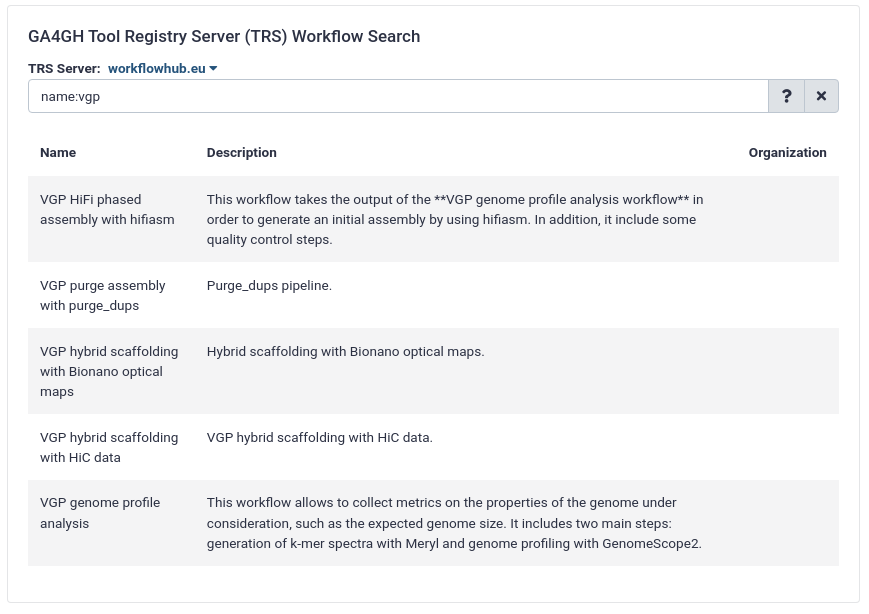
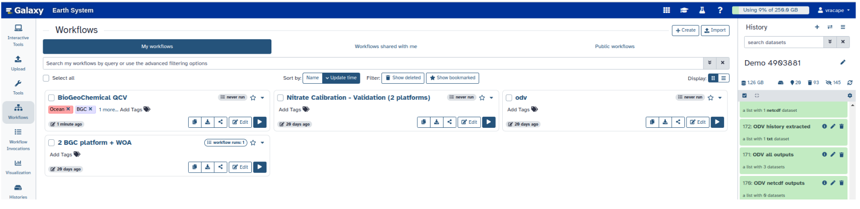
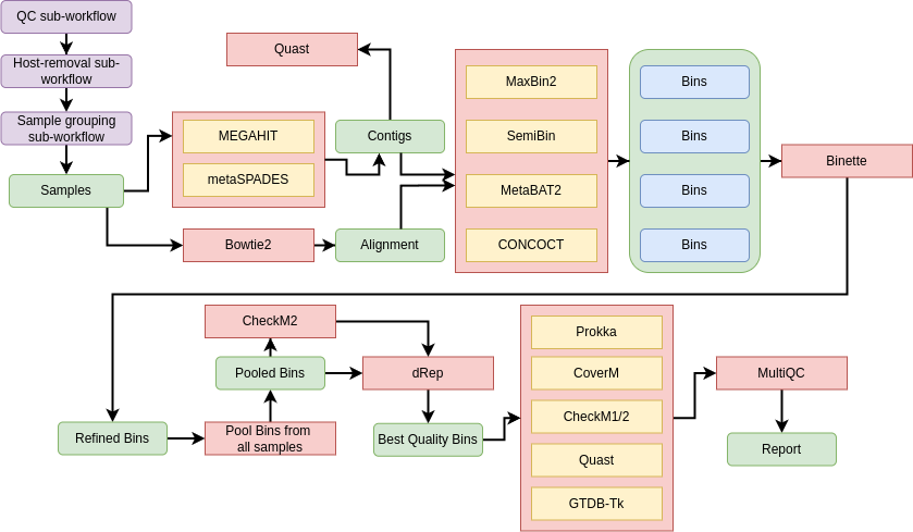
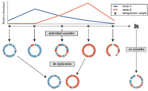 Open image in new tab
, Mash ANI is severely impacted. Source: <a href='https://drep.readthedocs.io/en/latest/choosing_parameters.html#importance-of-genome-completeness'>dRep documentation</a>")

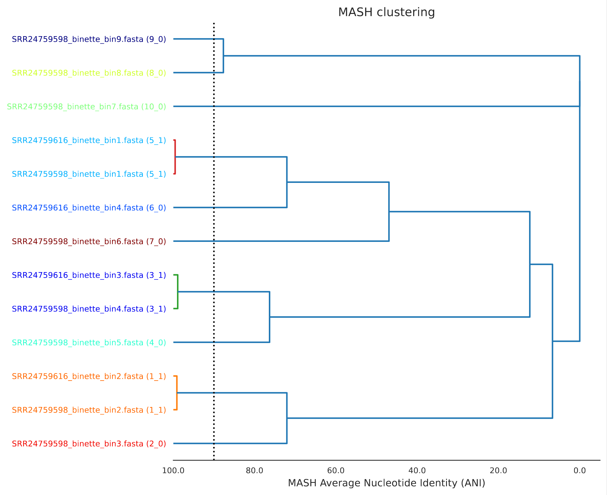
Open image in new tab