This tutorial is designed to guide you through the Ecoregionalization Galaxy workflow, demonstrating how to create an ecoregionalization map from occurrences and environmental data using a boosted regression trees model for predictions.
The workflow, consisting of six tools, is intended for processing occurrence data, which should include latitude, longitude and species presence or absence. The tutorial will provide a detailed explanation of inputs, workflow steps, and outputs. This tutorial gives a practical example, highlighting a use case centered on the Dumont d’Urville sea region and benthic invertebrates.
The primary goal of this workflow is to generate species distribution maps and identify ecoregions within the study area. The project’s objective is to offer accessible, reproducible, and transparent IT solutions for processing and analyzing species occurrence data.
This workflow is therefore composed of 6 tools:
GeoNearestNeighbor
BRT prediction tool
TaxaSeeker
ClusterEstimate
ClaraClust
EcoMap
And in this tutorial we will be using 5 more tools to format data before running the ecoregionalization workflow:
Advanced cut
Column Regex Find And Replace
Filter Tabular
Merge Columns
Interactive JupyterLab and notebook
Let’s delve into the tutorial, outlining each step and tool to manage the creation of ecoregionalization maps.
Ecoregionalization: The process by which a territory is classified into a category of area that respond to the same environmental factors taking into account species information.
Occurrences data: Data showing the presence of a species at a particular location.
Environmental data: Environmental data are any measurement or information that describe environmental processes, location, or conditions.
Boosted regression trees (BRT): Boosted Regression Trees is a kind of regression methodology based on Machine Learning. Unlike conventional regression methods (GLMs, GAMs), BRTs combine numerous basic decision trees to enhance the predictive performance. BRTs can handle complex relationships and interactions among predictors, and it is considered a robust technique that can control outliers and nonlinearity.
Clustering: Clustering is a machine learning method of grouping data points by similarity or distance.
CLARA/PAM : CLARA (Clustering Large Applications), is an extension to k-medoids (PAM) methods to deal with data containing a large number of objects. PAM stands for “Partition Around Medoids”, the PAM algorithm searches for k representative objects in a data set (k medoids) and then assigns each object to the closest medoid in order to create clusters.
This part will present the type of data you need to run the ecoregionalization workflow. This data will be downloaded in the next part of the tutorial.
Environmental data
To run this workflow, you will first need environmental data. This workflow accepts several types of environmental parameters like temperature or soil type. However, there is a mandatory file format, the tabular format (.tsv), and each pixel of the study area must be described in this file by associating latitude and longitude with environmental parameters.
In the use case presented in this tutorial, seventeen abiotic and physical parameters of the Dumont D’Urville sea region are used. They were taken from oceanographic models and in situ measurements Hemery et al. 2011. The physical oceanographic parameters are mean temperature and its standard deviation, mean salinity and its standard deviation, mean current magnitude and its standard deviation, maximum current bearing, maximum current magnitude and sea ice production. Bathymetric parameters are depth, slope, and rugosity. Finally, the seabed substrate composition was characterized by percentages of biogenic carbonate, biogenic silica, gravel, sand, and mud.
Here an example of environmental file input:
long
lat
Carbo
Grav
…
139.22
-65.57
0.88
28.59
…
139.25
-65.63
0.88
28.61
…
…
…
…
…
…
Occurrence data
The second data file you will need to run this workflow is an occurrences data file. As defined above, occurrences data are showing the presence (1) or absence (0) of a species at a particular location. This data file also needs to be in tabular format (.tsv) and need to be construct as following:
latitude and longitude columns.
One column per taxon where each box corresponding to a geographical point is marked 1 if the taxon is present or 0 if the taxon is absent.
Here an example of occurrences data file input:
lat
long
Acanthorhabdus_fragilis
Acarnidae
…
-65,9
142,3
1
0
…
-66,3
141,3
0
1
…
…
…
…
…
…
For this tutorial, occurrences data from the Dumont d’Urville sea region will be downloaded from the GBIF. These data were collected as part of the CEAMARC program (The Collaborative East Antarctic Marine Census Hosie et al. 2011) between December 2007 and January 2008 Beaman et al. 2009. Prior to its inclusion in GBIF, these data originated from collections at the Muséum national d’Histoire naturelle (MNHN – Paris). A GBIF filter was used to download only the data of interest, namely the data from the CEAMARC expedition from the Aurora Australis icebreaker. The selected occurrences are invertebrates. In the GBIF query, five collections were selected: the cnidarians collection (IK), the echinoderm collection (IE), the crustaceans collection (IU), the molluscs collection (IM), and the tunicates collection (IT), and only occurrences recorded by “IPEV-AAD-MNHN” which correspond to the CEAMARC expedition.
Jupyter notebook for the interactive JupyerLab and notebook tool
To switch from the occurrence data download from GBIF to the occurrence data supported by the ecoregionalisation workflow, the final step of data preparation use the “Interactive JupyterLab and notebook” tool who needs a jupyter notebook to work. In this Jupyter notebook, we used the pivot_wider function of the tidyr R package to transform our data into a wider format and adapt it to subsequent analyses as part of the Galaxy workflow for ecoregionalization. This transformation allowed us to convert our data to a format where each taxon becomes a separate column. We also took care to fill in the missing values with zeros and to sum the individual counts in case of duplications. Then all data >= 1 are replaced by 1 to have only presence (1) or abscence (0) data.
Get data
Hands On: Data Upload
Create a new history for this tutorial and give it a name (example: “Ecoregionalization workflow”) for you to find it again later if needed.
To create a new history simply click the new-history icon at the top of the history panel:
Click on galaxy-pencil (Edit) next to the history name (which by default is “Unnamed history”)
Type the new name
Click on Save
To cancel renaming, click the galaxy-undo “Cancel” button
If you do not have the galaxy-pencil (Edit) next to the history name (which can be the case if you are using an older version of Galaxy) do the following:
Click on Unnamed history (or the current name of the history) (Click to rename history) at the top of your history panel
Type the new name
Press Enter
Import occurrence data file from GBIF, environment file from InDoRES and Jupyter notebook file from InDoRES
Occurrence data file as a zip file where you will find “occurrence.txt”
Click galaxy-uploadUpload at the top of the activity panel
Select galaxy-wf-editPaste/Fetch Data
Paste the link(s) into the text field
Press Start
Close the window
As an alternative to uploading the data from a URL or your computer, the files may also have been made available from a Choose from repositories:
Click on Upload Data on the top of the left panel
Click on Choose from repository and scroll down to find your repository or type the repository name in the search box on the top.
Select the datasets you want to import
click on OK
Click on Start
Click on Close
You can find the dataset has begun loading in you history.
The GBIF link allows you to download a zip file containing multiple information files about the dataset. The file that you need is the ‘occurrence.txt’ file that we will specifically extract on Galaxy in the following step.
Use Unzip a file ( Galaxy version 6.0+galaxy0) to create a data collection in your history where all GBIF archive files will be unzipped
Unhide the “occurence.txt” data file then modify datatype to select the “tabular” one
If your history contains hidden datasets you will see galaxy-show-hidden“Include hidden” button directly above the dataset display.
To un-hide datasets:
Type visible:hidden in the search box
Select datasets you want to un-hide
Click the dropdown that would appear at the top of the history;
Select “Unhide” option.
Alternatively, you can:
click galaxy-show-hidden“Include hidden” button directly above dataset display. This will cause hidden datasets to appear in history along with normal (un-hidden) datasets;
hidden datasets are distinguished by having galaxy-show-hidden within dataset box. Clicking on this icon will un-hide a given dataset;
Click on the galaxy-pencilpencil icon for the dataset to edit its attributes
In the central panel, click galaxy-chart-select-dataDatatypes tab on the top
In the galaxy-chart-select-dataAssign Datatype, select tabular from “New Type” dropdown
Tip: you can start typing the datatype into the field to filter the dropdown menu
Click the Save button
Rename the datasets if needed, notably “9756” by “pivot_wider_jupytool_notebook.ipynb” and “9777” by “ceamarc_env.tab”.
Click on the galaxy-pencilpencil icon for the dataset to edit its attributes
In the central panel, change the Name field
Click the Save button
Check that the datatype of the environment file and occurrence file are tabular.
Click on the galaxy-pencilpencil icon for the dataset to edit its attributes
In the central panel, click galaxy-chart-select-dataDatatypes tab on the top
In the galaxy-chart-select-dataAssign Datatype, select tabular from “New Type” dropdown
Tip: you can start typing the datatype into the field to filter the dropdown menu
Click the Save button
Data formatting
The first step of this tutorial is data formatting because the GBIF species occurrence file download needs to be in a specific format to be included inside the Ecoregionalization workflow.
Keep data columns that we need with Advanced Cut
Hands On: Select the columns we need
Advanced Cut ( Galaxy version 9.3+galaxy1) with the following parameters:
param-file“File to cut”: occurrence (Input dataset)
The columns we kept are : indivdualCount, decimalLatitude, decimalLongitude, phylum, class, order, family, genus, specificEpithet.
Replace empty space with NAs with Column Regex Find And Replace
This step is used to add NAs to replace empty space in the file. We will do that for the four first columns and then remove lines with NA to have a complete dataset.
Hands On: Replace empty space by NAs for the first column
Column Regex Find And Replace ( Galaxy version 1.0.3) with the following parameters:
param-file“Select cells from”: output (output of Advanced Cuttool)
“using column”: c1
In “Check”:
param-repeat“Insert Check”
“Find Regex”: ^$
“Replacement”: NA
Warning: Pay attention to the regex parameter
The regular expression (“^$”) is used to capture empty cells in the dataframe so that they can be replaced by NA (Not Available). It is not advised to modify this regular expression nor its replacement, as you will encounter problems while running the next parts of the workflow.
Hands On: Replace empty space by NAs for the second column
Column Regex Find And Replace ( Galaxy version 1.0.3) with the following parameters:
param-file“Select cells from”: out_file1 (output of Column Regex Find And Replace on the first columntool)
“using column”: c2
In “Check”:
param-repeat“Insert Check”
“Find Regex”: ^$
“Replacement”: NA
Hands On: Replace empty space by NAs for the third column
Column Regex Find And Replace ( Galaxy version 1.0.3) with the following parameters:
param-file“Select cells from”: out_file2 (output of Column Regex Find And Replace on the second columntool)
“using column”: c3
In “Check”:
param-repeat“Insert Check”
“Find Regex”: ^$
“Replacement”: NA
Hands On: Replace empty space by NAs for the fourth column
Column Regex Find And Replace ( Galaxy version 1.0.3) with the following parameters:
param-file“Select cells from”: out_file3 (output of Column Regex Find And Replace on the third columntool)
“using column”: c4
In “Check”:
param-repeat“Insert Check”
“Find Regex”: ^$
“Replacement”: NA
Check your output. At the end of this step you must have NA instead of empty space. See example below.
Figure 2: Output of Regex Find And Replace example
Merge taxa columns with Merge Columns
Hands On: Merge columns “phylum”, “class”, "order", "family", "genus" and "specificEpithet"
Merge Columns ( Galaxy version 1.0.2) with the following parameters:
param-file“Select data”: out_file1 (output of Column Regex Find And Replace on genus columntool)
“Merge column”: c4
“with column”: c5
In “Columns”:
param-repeat“Insert Columns”
“Add column”: c6
param-repeat“Insert Columns”
“Add column”: c7
param-repeat“Insert Columns”
“Add column”: c8
param-repeat“Insert Columns”
“Add column”: c9
Check your output. Your table must have a new column filled with the concatenation of “phylum”, “class”, “order”, “family”, “genus” and “specificEpithet” columns.
Remove columns no longer needed with Advanced Cut
Hands On: Remove columns that we don't need anymore
Advanced Cut ( Galaxy version 9.3+galaxy1) with the following parameters:
param-file“File to cut”: out_file (output of Merge Columnstool)
“Operation”: Discard
“Cut by”: fields
“Delimited by”: Tab
“Is there a header for the data’s columns ?”: Yes
“List of Fields”: c['4', '5', '6', '7', '8', '9']
Check your output. Columns “phylum”, “class”, “order”, “family”, “genus” and “specificEpithet” must have been deleted and your table must have four columns : “individualCount”, “decimalLatitude”, “DecimalLongitude” and “phylum_class_order_family_genus_specificEpithet”. See example below.
Obtain final data file with Interactive JupyterLab Notebook
The interactive JupyterLab Notebook allows to create, run, and share custom Galaxy tools based upon Jupyter Notebooks. Galaxy offers you to use Jupyter Notebooks directly in Galaxy accessing and interacting with Galaxy datasets as you like.
Here you will load an existing jupyter notebook (“pivot_wider_jupytool_notebook.ipynb” that you downloaded earlier) and run the code in it to get the final file that is needed for ecoregionalization workflow.
Hands On: Pivot_wider with Jupytool
Interactive JupyterLab and notebook with the following parameters:
“Do you already have a notebook?”: Load a previous notebook
param-file“Select value”: output (output of previous step Advanced Cuttool)
Warning: Pay attention to the tool version
It is possible to have specific troubleshoots with using interactive tools as, for now, we can’t redirect to a specific version of the tool (as for classical tool) from the tutorial page. Here, if you encounter errors, you maybe need to specify the 1.0.0 version (the one used for the tuto) !
The first parameter allows you to specify that you want to use a previous notebook (“pivot_wider_jupytool_notebook.ipynb”) rather than create a new one.
Then you need to insert your ready to use jupyter notebook (“pivot_wider_jupytool_notebook.ipynb”).
The third parameter is important to specify that you just want to execute a notebook and not dive into the web frontend (in this case).
Then you need to clik on “+ Insert User inputs”” button to add the next parameters.
After, you need to give a name to your input and choose its type.
Finally you have to input the occurrence data file that will be treated in the Jupyter Notebook.
Figure 4: Interactive JupyterLab Notebook parameters example
Check your output (“Intercative JupyterLab Notebook on data (pivot_file)”) in your galaxy history. You must have a tabular file with latitude and longitude in first two columns and the others columns must be taxa. See example below.
Figure 5: Interactive JupyterLab Notebook output example
Warning: Galaxy can't display properly file with too many columns
Too avoid having web interface issues, Galaxy is not displaying tabulated files with “beautifull” columns visualization when number of clumns is big. That’s why here we are showing the preview of the dataset from the history.
Question
How many columns have your data file now?
It must have 202 columns.
Ecoregionalization workflow
Now you have all you need to run the ecoregionalization Workflow :
Occurrence formatted file
Environment file
Merge environment and occurence file with GeoNearestNeighbor
What it does ?
This Galaxy tool allows you to merge two data tables (tabular format only) according to their latitude and longitude coordinates (in WGS84 projection), finding the closest points. This tool is used in the Ecoregionalization workflow to filter the occurence data file so it can be used on the BRT prediction tool.
How to use it ?
Hands On: Run GeoNearestNeighbor
GeoNearestNeighbor ( Galaxy version 0.1.0+galaxy0) with the following parameters:
In “Your environment file (or table 1)”:
param-file“Input your environment data file (tabular format only)”: ceamarc_env.tsv (Input dataset)
“Choose columns where your latitude is in your environment data file.”: c2
“Choose columns where your longitude is in your environment data file.”: c1
In “Your occurrence file (or table 2)”:
param-file“Input your occurrence data file (tabular format only)”: pivot_file (output of Interactive JupyTool and notebooktool)
“Choose columns where your latitude is in your occurrence data file.”: c1
“Choose columns where your longitude is in your occurrence data file.”: c2
Comment: Coords precision
It is recommended that, for optimal precision, the latitude and longitude values in both files should be of the same precision level. And, for the sake of relevance, the geographical coordinates in both files should be as close as possible to apply the most accurate environmental parameters to the correct species occurrences
Check your outputs. You must have two files:
Information file containing the coordinates of occurrence data, the coordinates retains from environmental data and the distances between the two.
Occurrence and Environment merge file containing occurrence data and environmental data cooresponding.
Predicting taxa distribution with BRT tool prediction
This step implements a commonly used approach in ecological studies, namely species distribution modelling (SDM). This allows to characterize the distribution of each taxon by giving an indicator of probability of taxon presence for each environmental layer pixel. Here, the boosted regression trees (BRT) method was used to adjust the relationship between the presence of a single taxon and the environmental conditions under which the taxon has been detected. BRT modelling is based on an automatic learning algorithm using iterative classification trees.
What it does ?
Two treatments are performed in this tool: the creation of the taxa distribution model and the use of this model to obtain a prediction index. The prediction index obtained from each BRT model for each pixel of the environmental layers is an approximation of the probability of detection of the presence of the taxon.
This tool gives as output a file containing the predictions of the probability of the presence of each taxon for each “environment pixel” (latitude, longitude), a visualization of these pixels for each taxon and graphs showing the percentage of model explanation for each environmental parameter. We’re gonna go back to this in the following steps.
How to use it ?
Hands On: Run the BRT tool
BRT tool prediction ( Galaxy version 0.1.0+galaxy0) with the following parameters:
param-file“Input your environment data file of your study area (tabular format only)”: ceamarc_env.tsv (Input dataset)
param-file“Input your occurrences data file(s) containing also the environmental characteristics where the species has been observe (tabular format only)”: Merge table (output of GeoNearestNeighbortool)
Click on param-filesMultiple datasets
Select several files by keeping the Ctrl (or COMMAND) key pressed and clicking on the files of interest
“Choose column(s) where your abiotic parameter are in your environment data file.”: c['3', '4', '5', '6', '7', '8', '9', '10', '11', '12', '13', '14', '15', '16', '17', '18', '19']
Warning: You maybe can here prepare a cup of tea ;)
This step is a first “long” one, and you have to wait something like 18 minutes and 34 sec to obtain the result. It is maybe the good moment to have a break and go outside to admirate biodiversity around you?
Check your outputs. You must have four outputs collections.
Prediction files
Validation files (Taxa, AUC, Tree complexity, Total deviance explained)
Species distribution prediction maps
Partial dependence plots
In the ‘Prediction files’ collection there must be a file containing predictions of the probability of the presence of each taxon for each “environmental pixel” (latitude, longitude) for each occurrence file you entered.
In the ‘Validation files’ collection there must be a file containing for each taxon the validation metrics of the associated model.
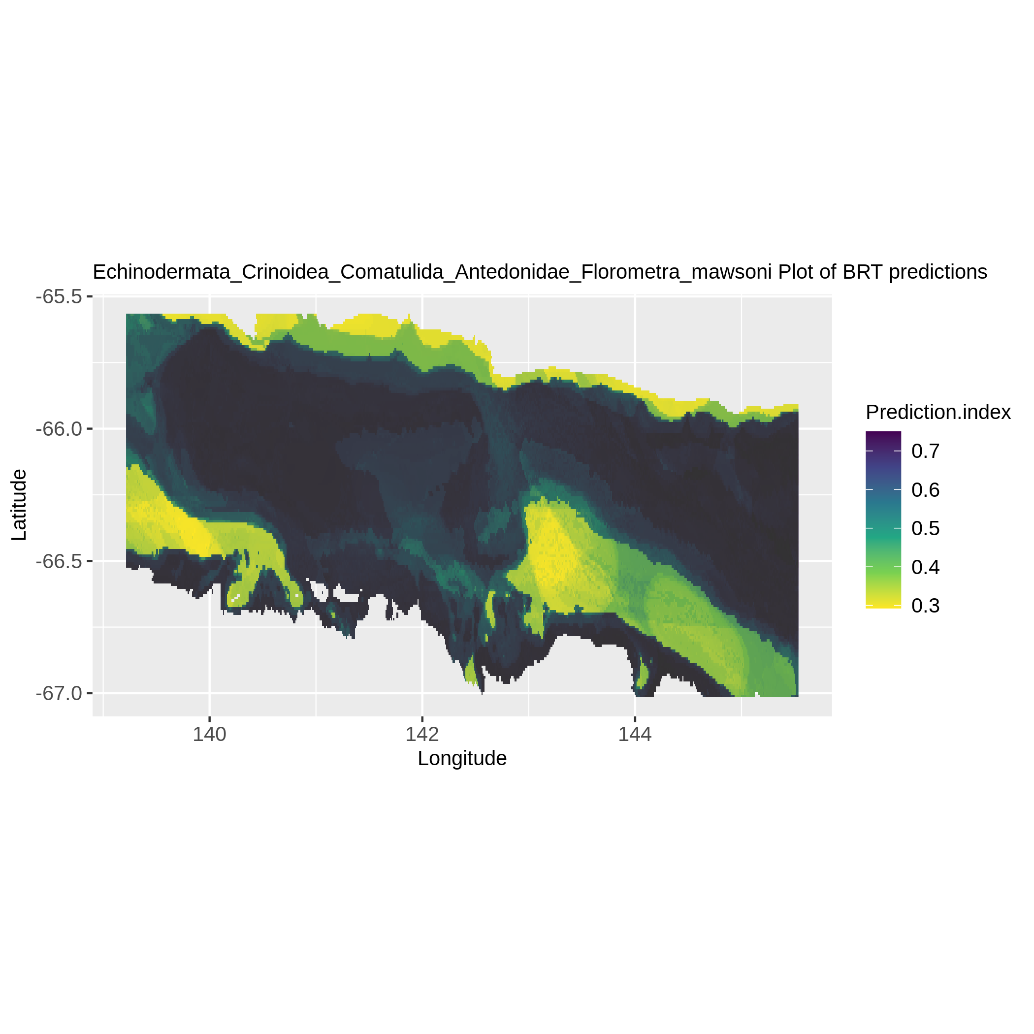
In the ‘Species distribution prediction maps’ collection there must be for each taxon a map representing their probability of presence at each environmental layer pixel.
Here is an example:
Figure 6: Florometra mawsoni distribution from BRT
In the ‘Partial dependence plots’ collection there should be graphs showing the percentage explanation of the model for each environmental parameter.
Here is an example:
Figure 7: Percentage of explanation of the model for each environmental parameter
Collecting the list of taxa with TaxaSeeker
What it does ?
This tool does three things:
It allows obtaining a summary file for each taxon indicating whether a BRT model was obtained and the number of occurrences per taxon.
It provides a list of taxa that obtained cleaned BRT models (without “_”, “_sp”, etc.) to propose the list to WoRMS (World Register of Marine Species) or another taxonomic database and obtain more information about the taxa.
It generates a list of taxa for which a BRT model was obtained, needed as input of following steps.
How to use it ?
Hands On: Run TaxaSeeker
TaxaSeeker ( Galaxy version 0.1.0+galaxy0) with the following parameters:
param-file“Environment file (tabular format only)”: ceamarc_env.tsv (Input dataset)
param-file“Occurences file(s) (tabular format only)”: Merged table (output of GeoNearestNeighbortool)
param-file“Predictions file(s)”: Prediction files collection (output of BRT tool predictiontool)
Click on param-collectionDataset collection in front of the input parameter you want to supply the collection to.
Select the collection you want to use from the list
Check your outputs. You must have three files:
Summary of taxa model
List of taxa
List of taxa clean
Determine the optimal number of clusters with ClusterEstimate
What it does ?
This tool enables the determination of the optimal number of clusters for partition-based clustering, along with generating files used in the following anlaysis steps.
The tool will produce three outputs. The first two files that will be used in the following steps of the workflow: a file containing four pieces of information (latitude, longitude, presence prediction and corresponding taxon), and a file containing the data to be partitioned.
The third output corresponds to the main information of the tool, a graph presenting the value of the SIH index according to the number of clusters. The silhouette index provides a measure of the separation between clusters and the compactness within each cluster. The silhouette index ranges from -1 to 1. Values close to 1 indicate that objects are well grouped and separated from other clusters, while values close to -1 indicate that objects are poorly grouped and may be closer to other clusters. A value close to 0 indicates a situation where objects are located at the border between two neighboring clusters. Thus the optimal number of clusters is the one that maximizes the value of the SIH index.
How to use it ?
Hands On: Run ClusterEstimate
ClusterEstimate ( Galaxy version 0.1.0+galaxy0) with the following parameters:
param-file“Environment file (tabular format only)”: ceamarc_env.tsv (Input dataset)
param-file“Taxa selected file (File ‘List of taxa’ from TaxaSeeker tool)”: List_of_taxa (output of TaxaSeekertool)
param-file“Prediction files”: Prediction files collection (output of BRT tool predictiontool)
Click on param-collectionDataset collection in front of the input parameter you want to supply the collection to.
Select the collection you want to use from the list
“Number of Cluster to test”: 10 (You can choose any number, but remember that the more cluster numbers to test the longer it will take)
Comment: Two other parameters
The other two parameters can be left as is. If you need to change them here is a short description of what they do:
The first one is metric used to calculate the dissimilarities between the observations: Manhattan (distance between two real-valued vectors), Euclidean (shortest distance between two
points) and Jaccard (defined as the size of the intersection divided by the size of the union of the sample sets)
The second one is the sample size that will be used to perform clustering.
Indeed, the clara function is used to cluster large data using a representative sample rather than the entire data set. This will speed up the clustering process and make the calculation
more efficient. A fairly high value representative of the data is recommended. It is important to note that using a too small sample size may result in loss of information compared to using the
entire data set.
Check your outputs. You must have three files:
SIH index plot (See example below)
Data to cluster (Containing the data to be partitioned)
Data.bio table (Containing four pieces of information, latitude, longitude, presence prediction and corresponding taxon)
Question
What is the optimal number of clusters in this use case ?
The optimal number of cluster is seven because it maximizes the value of the SIH index.
With this graph you will be able to determine the optimal number of clusters retained for the construction of ecoregions. As said before, the optimal number of cluster is the one that maximizes the SIH index. In this example, the number of clusters that optimizes the SIH index is seven.
Build ecoregional clusters with ClaraClust
What it does ?
After choosing an optimal number of clusters with the ClusterEstimate tool, we can now partition each latitude and longitude point according to their associated values of the BRT prediction index. Due to
the large size of the datasets, the Clara function of the Cluster package is used here to apply the Partitioning Around Medoids (PAM) algorithm on a representative sample of the data. This speeds up the
clustering process and makes the calculation more efficient.
How to use it ?
Hands On: Run ClaraClust
ClaraClust ( Galaxy version 0.1.0+galaxy0) with the following parameters:
param-file“Prediction matrix (file ‘data to cluster’ from Cluster Estimate tool)”: Data_to_cluster (output of ClusterEstimatetool)
param-file“Prediction table (file ‘data.bio table’ from Cluster Estimate tool)”: Data.bio_table (output of ClusterEstimatetool)
“Number of Cluster wanted”: 7 (Number of cluster determined at the previous step of the workflow in “SIH index plot”)
Comment: Two other parameters
The other two parameters can be left as is. If you need to change them here is a short description of what they do:
The first one is metric used to calculate the dissimilarities between the observations: Manhattan (distance between two real-valued vectors), Euclidean (shortest distance between two
points) and Jaccard (defined as the size of the intersection divided by the size of the union of the sample sets)
The second one is the sample size that will be used to perform clustering.
Indeed, the clara function is used to cluster large data using a representative sample rather than the entire data set. This will speed up the clustering process and make the calculation
more efficient. A fairly high value representative of the data is recommended. It is important to note that using a too small sample size may result in loss of information compared to using the
entire data set.
Check your outputs. You must have three files:
SIH index plot (See example below.)
Cluster points (Contains the latitude and longitude of each “environmental pixel” and the associated cluster number. We will use it in the next step of the workflow)
Cluster info (Contains all the information related to the clusters created, that is, in column: the latitude, the longitude, the corresponding cluster number and for each taxon the prediction value)
The tool will produce a silhouette plot that you can see below. A silhouette graph is a representation used to visualize the silhouette index of each observation in a clustered data set. It makes it possible to
assess the quality of clusters and determine their coherence and separation. In a silhouette graph, each observation is represented by a horizontal bar whose length is proportional to its silhouette index. The longer
the bar, the better the consistency of the observation with its cluster and the separation from other clusters. As mentioned above, the silhouette index ranges from -1 to 1. Values close to 1 indicate that objects
are well grouped and separated from other clusters, while values close to -1 indicate that objects are poorly grouped and may be closer to other clusters. A value close to 0 indicates a situation where objects are
located at the border between two clusters. Here, in the graph below, there is a good distribution of the observations because the majority of the bars are above the average value of the silhouette index.
Congratulations! You have successfully completed the ecoregionalization workflow. Here is the end of this tutorial aiming to explain the purpose of the ecoregionalization workflow and how to use it. This workflow provides a systematic and reproducible approach to ecoregionalization, allowing researchers to identify distinct ecological regions based on species occurrences and environmental data. This tutorial shows how to use this workflow, step by step, or all in one using the Dumont D’Urville sea region use case with related datasets. It allows you to understand ecoregions construction. You learned the use of the BRT algorithm for modeling species distribution as well as the cluster construction with the k-medoid clustering algorithms (CLARA/PAM). Feel free to explore and adapt this workflow for your specific research needs. If you have any questions, or encounter issues during the workflow, refer to the provided documentation or seek assistance from the Galaxy community. Don’t hesitate to contact us if you have any questions.
You've Finished the Tutorial
Please also consider filling out the Feedback Form as well!
Key points
Get raw data from research data wharehouse
Clean data content to be used by an existing workflow
Evaluate the best number of cluster to cut a dataset
Frequently Asked Questions
Have questions about this tutorial? Have a look at the available FAQ pages and support channels
Further information, including links to documentation and original publications, regarding the tools, analysis techniques and the interpretation of results described in this tutorial can be found here.
Hemery, L. G., B. Galton-Fenzi, N. Améziane, M. J. Riddle, S. R. Rintoul et al., 2011 Predicting habitat preferences for Anthometrina adriani (Echinodermata) on the East Antarctic continental shelf. Marine Ecology Progress Series 441: 105–116. 10.3354/meps09330
Hosie, G., P. Koubbi, M. Riddle, C. Ozouf-Costaz, M. Moteki et al., 2011 CEAMARC, the Collaborative East Antarctic Marine Census for the Census of Antarctic Marine Life (IPY # 53): An overview. Polar Science 5: 75–87. 10.1016/j.polar.2011.04.009
Feedback
Did you use this material as an instructor? Feel free to give us feedback on how it went.
Did you use this material as a learner or student? Click the form below to leave feedback.
Hiltemann, Saskia, Rasche, Helena et al., 2023 Galaxy Training: A Powerful Framework for Teaching! PLOS Computational Biology 10.1371/journal.pcbi.1010752
Batut et al., 2018 Community-Driven Data Analysis Training for Biology Cell Systems 10.1016/j.cels.2018.05.012
@misc{ecology-Ecoregionalization_tutorial,
author = "Pauline Seguineau",
	title = "Ecoregionalization workflow tutorial (Galaxy Training Materials)",
	year = "",
	month = "",
	day = "",
	url = "\url{https://training.galaxyproject.org/training-material/topics/ecology/tutorials/Ecoregionalization_tutorial/tutorial.html}",
	note = "[Online; accessed TODAY]"
}
@article{Hiltemann_2023,
	doi = {10.1371/journal.pcbi.1010752},
	url = {https://doi.org/10.1371%2Fjournal.pcbi.1010752},
	year = 2023,
	month = {jan},
	publisher = {Public Library of Science ({PLoS})},
	volume = {19},
	number = {1},
	pages = {e1010752},
	author = {Saskia Hiltemann and Helena Rasche and Simon Gladman and Hans-Rudolf Hotz and Delphine Larivi{\`{e}}re and Daniel Blankenberg and Pratik D. Jagtap and Thomas Wollmann and Anthony Bretaudeau and Nadia Gou{\'{e}} and Timothy J. Griffin and Coline Royaux and Yvan Le Bras and Subina Mehta and Anna Syme and Frederik Coppens and Bert Droesbeke and Nicola Soranzo and Wendi Bacon and Fotis Psomopoulos and Crist{\'{o}}bal Gallardo-Alba and John Davis and Melanie Christine Föll and Matthias Fahrner and Maria A. Doyle and Beatriz Serrano-Solano and Anne Claire Fouilloux and Peter van Heusden and Wolfgang Maier and Dave Clements and Florian Heyl and Björn Grüning and B{\'{e}}r{\'{e}}nice Batut and},
	editor = {Francis Ouellette},
	title = {Galaxy Training: A powerful framework for teaching!},
	journal = {PLoS Comput Biol}
}
Funding
These individuals or organisations provided funding support for the development of this resource
Questions:

Open image in new tab
Open image in new tab
Open image in new tab
Open image in new tab
Open image in new tab
 Open image in new tab
 Open image in new tab
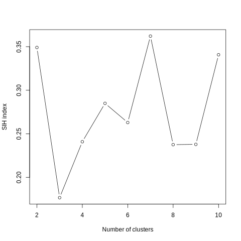 Open image in new tab
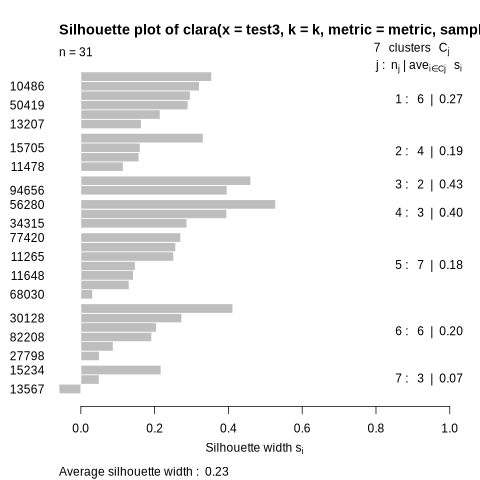 Open image in new tab
 Open image in new tab