Use Jupyter notebooks in Galaxy
| Author(s) |
|
| Editor(s) |
|
| Tester(s) |
|
| Reviewers |
|
OverviewQuestions:
Objectives:
How to open a Jupyter Notebook in Galaxy?
How to update dependencies in a Jupyter Interactive Environment?
How to save and share results in the Galaxy History?
Requirements:
Learn about the Jupyter Interactive Environment
Load data into a Jupyter Interactive Environment
Install library dependencies
Save a notebook to the Galaxy history
- tutorial Hands-on: Galaxy Basics for genomics
- tutorial Hands-on: Understanding Galaxy history system
Time estimation: 1 hourLevel: Introductory IntroductorySupporting Materials:Published: Jul 2, 2018Last modification: Dec 17, 2025License: Tutorial Content is licensed under Creative Commons Attribution 4.0 International License. The GTN Framework is licensed under MITpurl PURL: https://gxy.io/GTN:T00148rating Rating: 4.7 (3 recent ratings, 14 all time)version Revision: 11
In this tutorial, we are going to explore the basics of using JupyterLab in Galaxy. We will use the Gapminder data as a test set to get the hang of Jupyter notebooks. The python-novice-gapminder-data.zip file is publicly available. This tutorial can also be used as an initial setup for the Software Carpentries training Plotting and Programming in Python.
AgendaIn this tutorial, we will see :
What is Jupyter?
Jupyter is an interactive environment that mixes explanatory text, command line and output display for an interactive analysis environment. Its implementation in Galaxy facilitates the performance of additional analyses if there are no tools for it.
These notebooks allow you to replace any in-house script you might need to complete your analysis. You don’t need to move your data out of Galaxy. You can describe each step of your analysis in the markdown cells for an easy understanding of the processes, and save it in your history for sharing and reproducibility. In addition, thanks to Jupyter magic commands, you can use several different languages in a single notebook.

You can find the complete manual for Jupyter commands on Read the Docs.
Use Jupyter notebook in Galaxy
Import data
To manipulate data, we first upload the python-novice-gapminder-data.zip folder into your Galaxy history. To add the files, you can either upload them locally from your computer or use Zenodo. To add the files, you can either upload them locally from your computer or use Zenodo.
Hands On: Data upload using Zenodo
Create a new history for this Jupyter notebook exercise
To create a new history simply click the new-history icon at the top of the history panel:
Import the following tabular file from Zenodo:
https://zenodo.org/record/15263830/files/gapminder_all.csv
https://zenodo.org/record/15263830/files/gapminder_gdp_africa.csv
https://zenodo.org/record/15263830/files/gapminder_gdp_americas.csv
https://zenodo.org/record/15263830/files/gapminder_gdp_asia.csv
https://zenodo.org/record/15263830/files/gapminder_gdp_europe.csv
https://zenodo.org/record/15263830/files/gapminder_gdp_oceania.csv
- Copy the link location
Click galaxy-upload Upload at the top of the activity panel
- Select galaxy-wf-edit Paste/Fetch Data
Paste the link(s) into the text field
Press Start
- Close the window
Make sure the files are imported as
CSVby expanding the box of each imported file in your history and check the format.
- Click on the galaxy-pencil pencil icon for the dataset to edit its attributes
- In the central panel, click galaxy-chart-select-data Datatypes tab on the top
- In the galaxy-chart-select-data Assign Datatype, select
csvfrom “New Type” dropdown
- Tip: you can start typing the datatype into the field to filter the dropdown menu
- Click the Save button

Open the JupyterLab environment
Opening up your JupyterLab:
Hands On: Launch JupyterLabCurrently JupyterLab in Galaxy is available on Live.useGalaxy.eu, usegalaxy.org and usegalaxy.eu.
Hands On: Run JupyterLab
- Interactive Jupyter Notebook. Note that on some Galaxies this is called Interactive JupyTool and notebook:
- Click Run Tool
The tool will start running and will stay running permanently
This may take a moment, but once the
Executed notebookin your history is orange, you are up and running!- On the left menu bar you should see the Interactive Tools Icon now. Click on it to open the Active Interactive Tools and locate the JupyterLab instance you started.
- Click on your JupyterLab instance (JupyTool interactive tool)
If JupyterLab is not available on the Galaxy instance:
- Start Try JupyterLab
You should now be looking at a page with the JupyterLab interface:

As shown in the figure above, JupyterLab interface is made of 3 main areas:
- The menu bar at the top
- The left side bar with, in particular, the File Browser
- The main work area in the central panel
Start your first notebook
Now that we are ready to start exploring JupyterLab, let’s open a python Notebook. There will be one pre-opened notebook available in the file browser on the left side called ipython_galaxy_notebook.ipynb. For this training, however, we will open a new Jupyter notebook, select a kernel and give it a name.
Hands On: Start a notebook
Open a new Jupyter notebook
There is more than one option to open a Jupyter notebook. One option is:
- Click on File in the top menu bar
- Select New -> Notebook
- Choose the kernel
Python 3 (ipykernel)from the dropdown menu and click selectChange the kernel (only if you run
JupyterLabwith Galaxy Version 1.0.1)If the kernel
Python [conda env:python-kernel-3.12]was chosen in the previous step, it should appear in the upper right corner of the notebook file. If not, this is the location where the kernel can be switched.
- Click on the field that displays the current kernel e.g.
Python [conda env:base]- Now select the kernel
Python [conda env:python-kernel-3.12]from the drop down menuName the Jupyter notebook
There are several options how to name or rename your Jupyter Notebook. One way is to:
- Click on File and select Save File As…
- Enter your file name e.g.
first_galaxy_notebook.ipynb. Note that your file needs to end with.ipynb- Click on Save
Install and import libraries using Conda
Some dependencies or programming libraries may not be available in the kernel your Jupyter Notebook is using. If that’s the case, you can install or update these libraries using Conda.
Hands On: Install from a Conda recipe
- Click on a cell of your notebook to edit it (verify that it is defined as a
Codecell)- Enter the following lines :
!conda install -y pandas
!conda install -y seaborn
- The
!indicates you are typing a bash command line (alternatively, you can add the line%%bashat the beginning of your cell. In that case, the whole cell will be run as bash commands.)
- The
-yoption allows the installation without asking for confirmation (The confirmation is not managed well by notebooks)shift+returnto run the cell or click on the run cell button.
If you wish to follow the Software Carpentries training Plotting and Programming in Python after finishing this Jupyter Notebook introduction, you should install the following Python libraries.
Hands On: Install Python libraries for a Python introduction
- Copy the following install commands and paste them into an empty cell of your Notebook
!conda install -y math !conda install -y matplotlib !conda install -y glob !conda install -y pathlib- press
shift+returnto run the cell or click on the run cell button.
Now you will be able to import these Python libraries and use them with your library code.
Hands On: Import Python libraries
Click on a cell of your notebook to edit it (verify that it is defined as a
Codecell)- Enter the following lines :
import pandas as pd import seaborn as sns from IPython.display import display import matplotlib.pyplot as pltshift+returnto run the cell or click on the run cell button.
Import data
If you want to include datasets from your history into your Jupyter notebook, you can import them using the get("[file_number]") command, with the number of your dataset in the history (If you are working on a collection, unhide datasets to see their numbers).
You can use the gapminder_gdp_europe.csv file. Using the get("[file_number]") function will retrieve or get the location where the dataset from your galaxy history (with the file_number) is stored. Within your Python program this file can be read using the location retrieved the get() function.
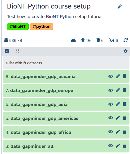
Looking at the history in the image you would need to call get("7") to get the file path of the gapminder_gdp_europe.csv file.
Hands On: Import a file location from your historySave the import file location to a variable (
file_import) name with theget()function.file_import = get("[file_number]")
- The files are referenced in Jupyter by their number in the history.
- The variable
file_importnow stores the location where your file can be imported from.
If you wish to follow the python training later you should import all of the gapminder datasets now. The file_import variables can be treated like the path with the tutorial.
Hands On: Import the training data locations from your history
- Find the
file_numbersof all of the gapminder datasets (gapminder_all.csv,gapminder_gdp_africa.csv,gapminder_gdp_americas.csv,gapminder_gdp_asia.csv,gapminder_gdp_europe.csv,gapminder_gdp_oceania.csv) with your galaxy history- Load the datasets
file_importinto your Ipython notebook:gapminder_all_import = get("[file_number]") gapminder_gdp_africa_import = get("[file_number]") gapminder_gdp_americas_import = get("[file_number]") gapminder_gdp_asia_import = get("[file_number]") gapminder_gdp_europe_import = get("[file_number]") gapminder_gdp_oceania_import = get("[file_number]")
- The files are referenced in Jupyter by their number in the history.
- The variable
file_importnow stores the location where your file can be imported from
Graph Display in Jupyter
In this tutorial, we are going to plot a distribution graph of our data. For this, we will first need to load one of our tabular data files. You can use the gapminder_all.csv file.
Hands On: Load a file from your history
- Open the dataset as a pandas DataFrame with the function.
dataframe = pd.read_csv(file_import)
- The files are referenced in Jupyter by their number in the history.
Hands On: Draw a distribution plot
- Create your figure with the command
fig, ax = plt.subplots(nrows=1, ncols=1, figsize=(15, 10))
nrows=1, ncols=1means you will have one plot in your figure (one row and one column)figsizeparameter determines the size of the figure- Draw the distribution plot of the second column of our dataset with the command
sns.histplot(data=dataframe, x='gdpPercap_1997', kde=True, ax=ax)

Export Data
If you want to save a file you generated in your notebook, use the put("file_name") command. That is what we are going to do with our distribution plot.
Hands On: Save a Jupyter-generated image into a Galaxy History
- Create an image file with the figure you just drew with the command
fig.savefig('distplot.png')- Export your image to your history with the command
put('distplot.png')
Save the Notebook in your history
Once you are done with your analysis or anytime during the editing process, you can save the notebook to your history using the put("first_galaxy_notebook.ipynb"). If you create additional notebooks with different names, make sure you save them all before you quit JupyterLab.
This will create a new notebook .ipynb file in your history every time you click on this icon.
Hands On: Closing JupyterLab
In the Galaxy interface, click on Interactive Tools button on the left side.
Tick galaxy-selector the box of your Jupyter Interactive Tool, and click Stop.
If you want to reopen a Jupyter Notebook saved in your history, you can use the tool Interactive JupyterLab Notebook, select “Load a previous Notebook”, and select the notebook from your history.
Conclusion
trophy You have just performed your first analysis in a Jupyter notebook integrated environment in Galaxy. You generated a distribution plot that you saved in your history along with the notebook to generate it.
If you wish to follow the Software Carpentries training Plotting and Programming in Python training now, you can open a Jupyter notebook install all needed dependencies and upload all file locations from the Gapminder dataset using the get('file_number') function (e.g. gapminder_all_file = get(12)). You can use this file location now throughout the tutorial once you need to specify the file path. Meaning, if the tutorial asks you to load a dataset like this data_oceania = pd.read_csv('data/gapminder_gdp_oceania.csv') you can replace the path 'data/gapminder_gdp_oceania.csv' with our file_import variable: data_oceania = pd.read_csv(gapminder_gdp_oceania_import).
You can start directly from The-jupyterlab-interface section of the tutorial.
You've Finished the Tutorial
Key points
Start Jupyter from the Visualize tab or from a dataset
Install Libraries with pip or Conda
Use get() to import datasets from your history to the notebook
Use put() to export datasets from the notebook to your history
Save your notebook in your history
Frequently Asked Questions
Have questions about this tutorial? Have a look at the available FAQ pages and support channelsFeedback
Did you use this material as an instructor? Feel free to give us feedback on how it went.
Did you use this material as a learner or student? Click the form below to leave feedback.

Citing this Tutorial
- Delphine Lariviere, Use Jupyter notebooks in Galaxy (Galaxy Training Materials). https://training.galaxyproject.org/training-material/topics/galaxy-interface/tutorials/galaxy-intro-jupyter/tutorial.html Online; accessed TODAY
- Hiltemann, Saskia, Rasche, Helena et al., 2023 Galaxy Training: A Powerful Framework for Teaching! PLOS Computational Biology 10.1371/journal.pcbi.1010752
- Batut et al., 2018 Community-Driven Data Analysis Training for Biology Cell Systems 10.1016/j.cels.2018.05.012
@misc{galaxy-interface-galaxy-intro-jupyter,
author = "Delphine Lariviere",
	title = "Use Jupyter notebooks in Galaxy (Galaxy Training Materials)",
	year = "",
	month = "",
	day = "",
	url = "\url{https://training.galaxyproject.org/training-material/topics/galaxy-interface/tutorials/galaxy-intro-jupyter/tutorial.html}",
	note = "[Online; accessed TODAY]"
}
@article{Hiltemann_2023,
	doi = {10.1371/journal.pcbi.1010752},
	url = {https://doi.org/10.1371%2Fjournal.pcbi.1010752},
	year = 2023,
	month = {jan},
	publisher = {Public Library of Science ({PLoS})},
	volume = {19},
	number = {1},
	pages = {e1010752},
	author = {Saskia Hiltemann and Helena Rasche and Simon Gladman and Hans-Rudolf Hotz and Delphine Larivi{\`{e}}re and Daniel Blankenberg and Pratik D. Jagtap and Thomas Wollmann and Anthony Bretaudeau and Nadia Gou{\'{e}} and Timothy J. Griffin and Coline Royaux and Yvan Le Bras and Subina Mehta and Anna Syme and Frederik Coppens and Bert Droesbeke and Nicola Soranzo and Wendi Bacon and Fotis Psomopoulos and Crist{\'{o}}bal Gallardo-Alba and John Davis and Melanie Christine Föll and Matthias Fahrner and Maria A. Doyle and Beatriz Serrano-Solano and Anne Claire Fouilloux and Peter van Heusden and Wolfgang Maier and Dave Clements and Florian Heyl and Björn Grüning and B{\'{e}}r{\'{e}}nice Batut and},
	editor = {Francis Ouellette},
	title = {Galaxy Training: A powerful framework for teaching!},
	journal = {PLoS Comput Biol}
}
Funding
These individuals or organisations provided funding support for the development of this resource
Congratulations on successfully completing this tutorial!
Do you want to extend your knowledge?Follow one of our recommended follow-up trainings:
You can use Ephemeris's
shed-tools installcommand to install the tools used in this tutorial.shed-tools install [-g GALAXY] [-a API_KEY] -t <(curl https://training.galaxyproject.org/training-material/api/topics/galaxy-interface/tutorials/galaxy-intro-jupyter/tutorial.json | jq .admin_install_yaml -r)Alternatively you can copy and paste the following YAML
---
install_tool_dependencies: true
install_repository_dependencies: true
install_resolver_dependencies: true
tools: []