JupyterLab in Galaxy
| Author(s) |
|
| Editor(s) |
|
| Reviewers |
|
OverviewQuestions:
Objectives:
How can I manipulate data using JupyterLab in Galaxy?
How can I start a notebook in JupyterLab?
How can I import/export dataset from/to my history to/from the notebook?
How can I save my notebook to my history?
Requirements:
Launch JupyterLab in Galaxy
Start a notebook
Import libraries
Use get() to import datasets from your history to the notebook
Use put() to export datasets from the notebook to your history
Save your notebook into your history
Time estimation: 1 hourSupporting Materials:Published: Mar 5, 2020Last modification: Apr 25, 2025License: Tutorial Content is licensed under Creative Commons Attribution 4.0 International License. The GTN Framework is licensed under MITpurl PURL: https://gxy.io/GTN:T00153rating Rating: 5.0 (0 recent ratings, 2 all time)version Revision: 9
JupyterLab is an Integrated Development Environment (IDE). Like most IDEs, it provides a graphical interface for R/Python, making it more user-friendly, and providing dozens of useful features. We will introduce additional benefits of using JupyterLab as you cover the lessons.
CommentThis tutorial is significantly based on the JupyterLab documentation “The JupyterLab Interface” section.
AgendaIn this tutorial, we will cover:
JupyterLab
Opening up your JupyterLab:
Hands On: Launch JupyterLabCurrently JupyterLab in Galaxy is available on Live.useGalaxy.eu, usegalaxy.org and usegalaxy.eu.
Hands On: Run JupyterLab
- Interactive Jupyter Notebook. Note that on some Galaxies this is called Interactive JupyTool and notebook:
- Click Run Tool
The tool will start running and will stay running permanently
This may take a moment, but once the
Executed notebookin your history is orange, you are up and running!- On the left menu bar you should see the Interactive Tools Icon now. Click on it to open the Active Interactive Tools and locate the JupyterLab instance you started.
- Click on your JupyterLab instance (JupyTool interactive tool)
If JupyterLab is not available on the Galaxy instance:
- Start Try JupyterLab
You should now be looking at a page with the JupyterLab interface:

As shown on the figure above, JupyterLab interface is made of 3 main areas:
- The menu bar at the top
- The left side bar with in particular the File Browser
- The main work area in the central panel
Start your first notebook
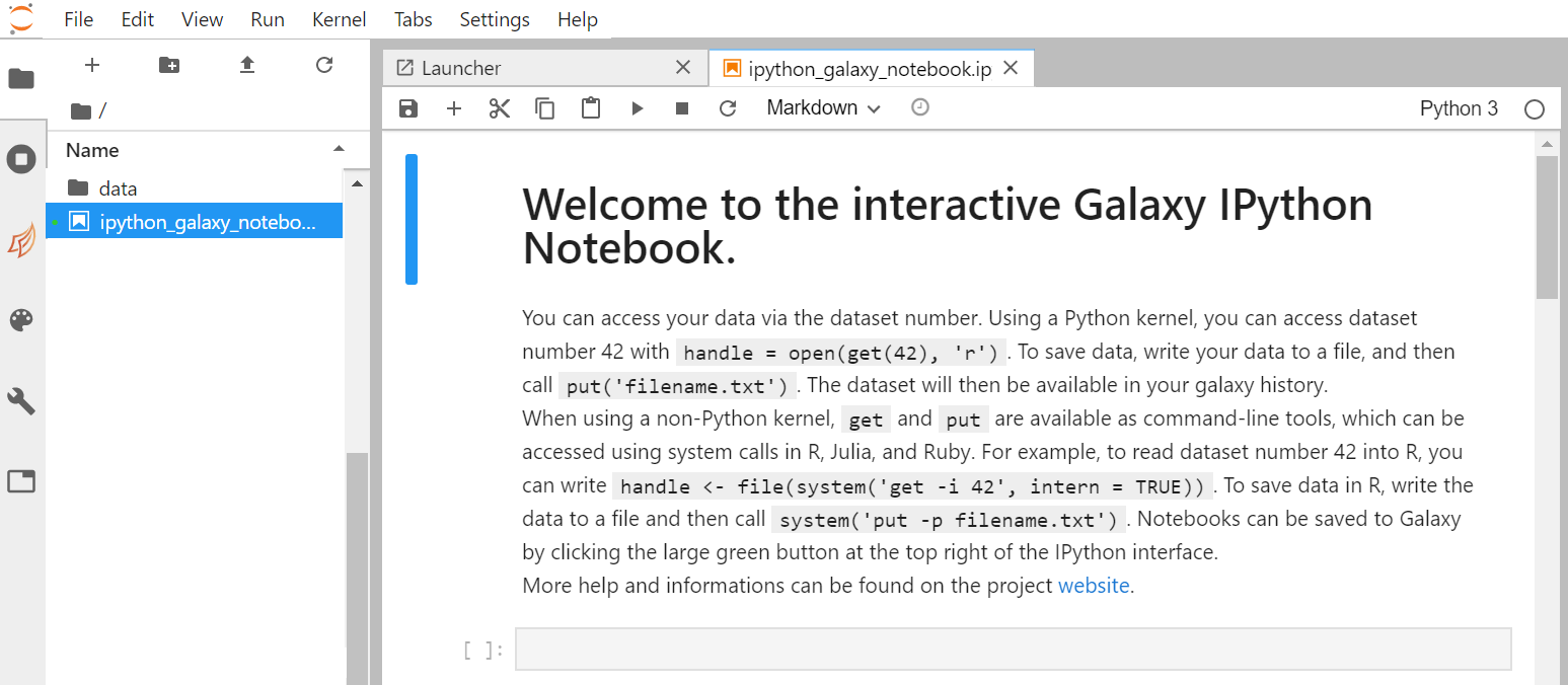
Now that we are ready to start exploring JupyterLab, we will want to keep a record of the commands we are using. To do this we can start a Notebook.
Hands On: Start a notebook
- On the left side bar, in the File Browser:
- Double-click on the file called ipython_galaxy_notebook.ipynb.
- Then select the default This will open the **Python [conda env:base] Kernel
- This will open a default notebook in the main work area.
- If ipython_galaxy_notebook.ipynb does not exist (for instance on Try JupyterLab), click on + (top left) to start The launcher. Then click on the Python icon in the Notebook section to create a new blank notebook.
A new notebook appears in the centre panel. Before we go any further, you should learn to save your script.
Hands On: Save a Python notebook
- There are several options to save your file:
- Click the File menu and select Save Notebook As….
- Click the galaxy-save icon (Save the notebook contents and create checkpoint) in the bar above the file tab line in the script editor.
- Click the File menu and select Save Notebook.
- Type CTRL+S (CMD+S on OSX).
- There are several options on how to (re-)name your file:
- After clicking on the option Save Notebook As, a window opens, where the file can be (re-)named.
- Right click on the current file name (
ipython_galaxy_notebook.ipynborUntitled.ipynb) in the bar above the first line in the script editor and select Rename Notebook in the opened selection window.- Alternatively, right click on the file name you would like to change on the left side in the folder menu. A window will open where you can select Rename.
The new script ipython_galaxy_notebook.ipynb should appear in the File Browser* in the left panel. By convention, Jupyter notebooks end with the file extension .ipynb independently of the programming language (R, Python, Octave, Julia, etc.).
Comment: Note: supported programming languagesDepending on your JupyterLab instance, the list of supported programming languages may vary. On Live.useGalaxy.eu, the following programming languages are currently supported:
- Python 3
- Julia
- R
- Octave
- Ansible
- Bash
- SciJava
By default, a Python notebook is started. Don’t worry if you are not familiar with Python programming language, it is not necessary for this tutorial. The same functionalities applies for any available programming languages.
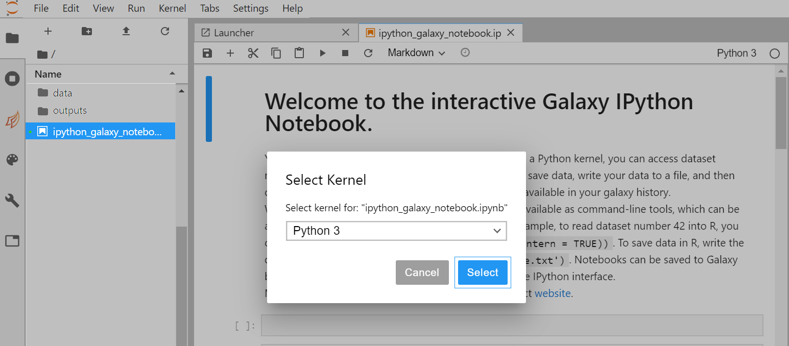
Comment: Note: switching to another programming languageOnce you have created a Notebook, you can switch to another available programming language (Switch Kernel).
- On the top right of your running Notebook, click on Python 3. A new window pops up:
- In this new window, click on Python 3 to select an available programming language (R, octave, Julia, etc.).
- Click on Select to activate your selection. The pop-up window closes and you are ready to use your notebook with the selected programming language. Alternatively, you can also:
- Click on + (top left menu) to start the Launcher. The list of available programming language is given in the Notebook section.
- Click on icon of your choice in the Notebook section.
- A new notebook is created with the programming language of your choice.
In the next step, we will create some visualizations. To visualize data, programming languages offer specific libraries. Before we use these libraries, we first need to ensure that these dependencies are installed.
Hands On: Install dependencies using Conda
- To open a console to install the dependencies, open the launcher window by clicking on the plus sign in the top-left corner. Within this window, click on
Python [conda env:python-kernel-3.12]iin the Console section.- After the console opens, you can enter the following lines into the cell at the bottom:
conda install -c conda-forge numpy matplotlib- Shift+Return to run the cell or click on the run cell button.
As the dependencies are installed within one Kernel the notebook needs to run on the same Kernel.
Hands On: Select Dernel
- First restart the Kernel, by clicking on Kernel in the upper menu and select Restart Kernel…
Next switch back to the your ipython notebook (e.g. ipython_galaxy_notebook.ipynb). You can find it next to the console tab on top of the right window.
- Below the taps you will find Python env button (e.g.
Python[conda env:base]). If you click on this one you can select a Kernel. Please select the Kernel, which was update in the previous step (Python [conda env:python-kernel-3.12]).
Now that the dependencies are installed and the Kernel is restarted, we can import the libraries.
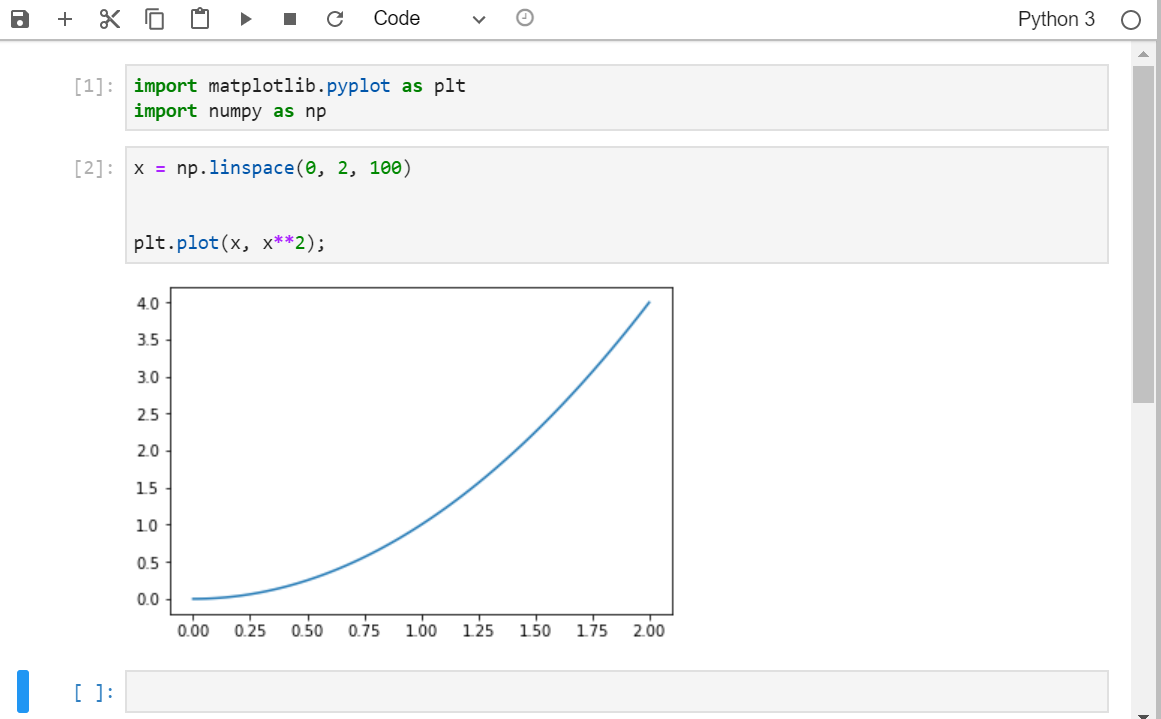
Hands On: Import Python libraries
- Click on a cell of your notebook to edit it (verify that it is defined as a “Code” cell)
- Enter the following lines:
import numpy as np import matplotlib.pyplot as plt- Shift+Return to run the cell or click on the run cell button.
Graph Display in JupyterLab with Python
In this tutorial we are going to simply plot a simple graph using generated data.
Hands On: Draw a simple plot
Generate a simple dataset
x = np.linspace(0, 2, 100)
y = x**2
Create your figure with the command:
fig, ax = plt.subplots( nrows=1, ncols=1 ,figsize=(15, 10) )
nrows=1, ncols=1means you will have one plot in your figure (one row and one column)figsizeparameter determine the size of the figureDraw the plot with the command
plt.plot(x, y);
Interaction between JupyterLab and Galaxy
Import / export Data
You can import data from Galaxy history using the get(12) command, with the number of your dataset in the history (If you are working on a collection, unhide datasets to see their numbers).
If you want to save a file you generated in your notebook, use the put("file_name") command. That is what we are going to do with our distribution plot.
Hands On: Save an Jupyter generated image into a Galaxy History
- Create an image file with the figure you just draw with the command
fig.savefig('simpleplot.png')- Export your image into your history with the command
put('simpleplot.png')
Save the Notebook in your history
Once you are done with you analysis or anytime during the editing process, you can save the notebook into your history using the put("ipython_galaxy_notebook.ipynb"). If you create additional notebooks with different names, make sure you save them all before you quit JupyterLab.
This will create a new notebook .pynb file in your history every time you click on this icon.
Hands On: Closing JupyterLab
In the Galaxy interface click on Interactive Tools button on the left side.
Tick galaxy-selector the box of your Jupyter Interactive Tool, and click Stop.
You've Finished the Tutorial
Key points
How to work with JupyterLab interactively within Galaxy
Frequently Asked Questions
Have questions about this tutorial? Have a look at the available FAQ pages and support channelsFeedback
Did you use this material as an instructor? Feel free to give us feedback on how it went.
Did you use this material as a learner or student? Click the form below to leave feedback.

Citing this Tutorial
- Anne Fouilloux, JupyterLab in Galaxy (Galaxy Training Materials). https://training.galaxyproject.org/training-material/topics/galaxy-interface/tutorials/jupyterlab/tutorial.html Online; accessed TODAY
- Hiltemann, Saskia, Rasche, Helena et al., 2023 Galaxy Training: A Powerful Framework for Teaching! PLOS Computational Biology 10.1371/journal.pcbi.1010752
- Batut et al., 2018 Community-Driven Data Analysis Training for Biology Cell Systems 10.1016/j.cels.2018.05.012
Congratulations on successfully completing this tutorial!@misc{galaxy-interface-jupyterlab, author = "Anne Fouilloux", title = "JupyterLab in Galaxy (Galaxy Training Materials)", year = "", month = "", day = "", url = "\url{https://training.galaxyproject.org/training-material/topics/galaxy-interface/tutorials/jupyterlab/tutorial.html}", note = "[Online; accessed TODAY]" } @article{Hiltemann_2023, doi = {10.1371/journal.pcbi.1010752}, url = {https://doi.org/10.1371%2Fjournal.pcbi.1010752}, year = 2023, month = {jan}, publisher = {Public Library of Science ({PLoS})}, volume = {19}, number = {1}, pages = {e1010752}, author = {Saskia Hiltemann and Helena Rasche and Simon Gladman and Hans-Rudolf Hotz and Delphine Larivi{\`{e}}re and Daniel Blankenberg and Pratik D. Jagtap and Thomas Wollmann and Anthony Bretaudeau and Nadia Gou{\'{e}} and Timothy J. Griffin and Coline Royaux and Yvan Le Bras and Subina Mehta and Anna Syme and Frederik Coppens and Bert Droesbeke and Nicola Soranzo and Wendi Bacon and Fotis Psomopoulos and Crist{\'{o}}bal Gallardo-Alba and John Davis and Melanie Christine Föll and Matthias Fahrner and Maria A. Doyle and Beatriz Serrano-Solano and Anne Claire Fouilloux and Peter van Heusden and Wolfgang Maier and Dave Clements and Florian Heyl and Björn Grüning and B{\'{e}}r{\'{e}}nice Batut and}, editor = {Francis Ouellette}, title = {Galaxy Training: A powerful framework for teaching!}, journal = {PLoS Comput Biol} }
You can use Ephemeris's
shed-tools installcommand to install the tools used in this tutorial.shed-tools install [-g GALAXY] [-a API_KEY] -t <(curl https://training.galaxyproject.org/training-material/api/topics/galaxy-interface/tutorials/jupyterlab/tutorial.json | jq .admin_install_yaml -r)Alternatively you can copy and paste the following YAML
---
install_tool_dependencies: true
install_repository_dependencies: true
install_resolver_dependencies: true
tools: []