Sequencing (determining of DNA/RNA nucleotide sequence) is used all over the world for all kinds of analysis. The product of these sequencers are reads, which are sequences of detected nucleotides. Depending on the technique these have specific lengths (30-500bp) or using Oxford Nanopore Technologies sequencing have much longer variable lengths.
Comment: Illumina MiSeq sequencing
Illumina MiSeq sequencing is based on sequencing by synthesis. As the name suggests, fluorescent labels are measured for every base that bind at a specific moment at a specific place on a flow cell. These flow cells are covered with oligos (small single strand DNA strands). In the library preparation the DNA strands are cut into small DNA fragments (differs per kit/device) and specific pieces of DNA (adapters) are added, which are complementary to the oligos. Using bridge amplification large amounts of clusters of these DNA fragments are made. The reverse string is washed away, making the clusters single stranded. Fluorescent bases are added one by one, which emit a specific light for different bases when added. This is happening for whole clusters, so this light can be detected and this data is basecalled (translation from light to a nucleotide) to a nucleotide sequence (Read). For every base a quality score is determined and also saved per read. This process is repeated for the reverse strand on the same place on the flow cell, so the forward and reverse reads are from the same DNA strand. The forward and reversed reads are linked together and should always be processed together!
Contemporary sequencing technologies are capable of generating an enormous volume of sequence reads in a single run. Nonetheless, each technology has its imperfections, leading to various types and frequencies of errors, such as miscalled nucleotides. These inaccuracies stem from the inherent technical constraints of each sequencing platform. When sequencing bacterial isolates, it is crucial to verify the quality of the data but also to check the expected species or strains are found in the data or if there is any contamination.
To illustrate the process, we take raw data of a bacterial genome (KUN1163 sample) from sequencing data produced in “Complete Genome Sequences of Eight Methicillin-Resistant Staphylococcus aureus Strains Isolated from Patients in Japan” (Hikichi et al. 2019).
Methicillin-resistant Staphylococcus aureus (MRSA) is a major pathogen
causing nosocomial infections, and the clinical manifestations of MRSA
range from asymptomatic colonization of the nasal mucosa to soft tissue
infection to fulminant invasive disease. Here, we report the complete
genome sequences of eight MRSA strains isolated from patients in Japan.
Any analysis should get its own Galaxy history. So let’s start by creating a new one and get the data (forward and reverse quality-controlled sequences) into it.
Hands On: Prepare Galaxy and data
Create a new history for this analysis
To create a new history simply click the new-history icon at the top of the history panel:
Rename the history
Click on galaxy-pencil (Edit) next to the history name (which by default is “Unnamed history”)
Type the new name
Click on Save
To cancel renaming, click the galaxy-undo “Cancel” button
If you do not have the galaxy-pencil (Edit) next to the history name (which can be the case if you are using an older version of Galaxy) do the following:
Click on Unnamed history (or the current name of the history) (Click to rename history) at the top of your history panel
Type the new name
Press Enter
Now, we need to import the data: 2 FASTQ files containing the reads from the sequencer.
Hands On: Import datasets
Import the files from Zenodo or from Galaxy shared data libraries:
Click galaxy-uploadUpload at the top of the activity panel
Select galaxy-wf-editPaste/Fetch Data
Paste the link(s) into the text field
Press Start
Close the window
As an alternative to uploading the data from a URL or your computer, the files may also have been made available from a shared data library:
Go into Libraries (left panel)
Navigate to the correct folder as indicated by your instructor.
On most Galaxies tutorial data will be provided in a folder named GTN - Material –> Topic Name -> Tutorial Name.
Select the desired files
Click on Add to Historygalaxy-dropdown near the top and select as Datasets from the dropdown menu
In the pop-up window, choose
“Select history”: the history you want to import the data to (or create a new one)
Click on Import
Rename the datasets to remove .fastqsanger.bz2 and keep only the sequence run ID (DRR187559_1 and DRR187559_2)
Click on the galaxy-pencilpencil icon for the dataset to edit its attributes
In the central panel, change the Name field to DRR187559_1
Click the Save button
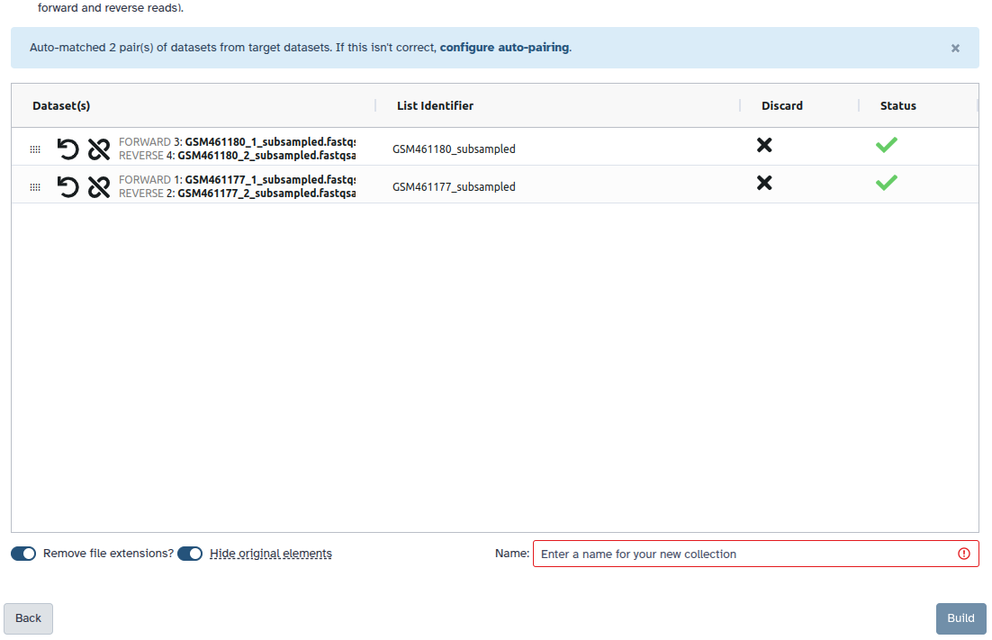
Create a paired collection named Paired Reads
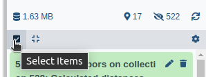
Click on galaxy-selectorSelect Items at the top of the history panel
Check all the datasets in your history you would like to include
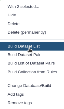
Click n of N selected and choose Advanced Build List
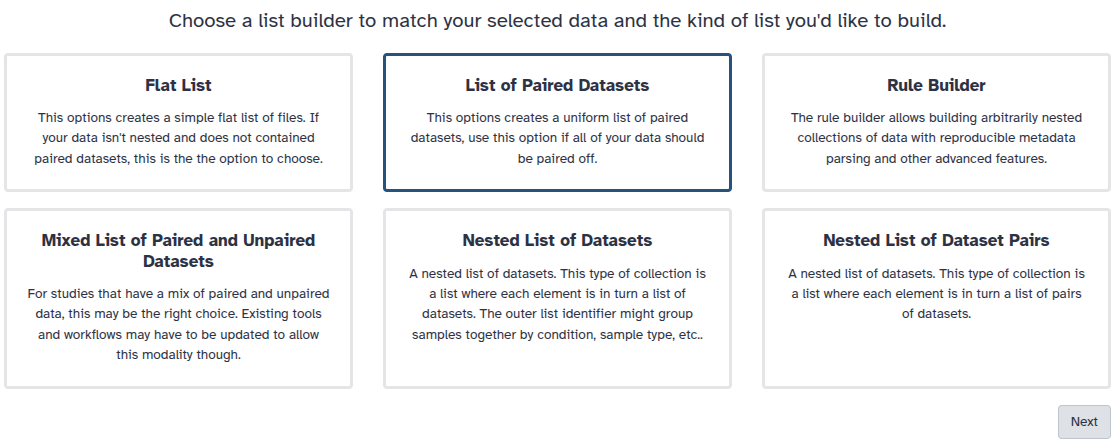
You are in the collection building wizard. Choose List of Paired Datasets and click ‘Next’ button at the right bottom corner.
Check and configure auto-pairing. Commonly matepairs have suffix _1 and _2 or _R1 and _R2. Click on ‘Next’ at the bottom.
Edit the List Identifier as required.
Enter a name for your collection
Click Build to build your collection
Click on the checkmark icon at the top of your history again
Tag the collection #unfiltered
Click on the collection in your history to view it
Click on Editgalaxy-pencil next to the collection name at the top of the history panel
Click on Add Tagsgalaxy-tags
Add a tag starting with #
Tags starting with # will be automatically propagated to the outputs any tools using this dataset.
Click Savegalaxy-save
Check that the tag appears below the collection name
Viewgalaxy-eye the renamed files in the collection
The datasets are both FASTQ files.
Question
What are the 4 main features of each read in a FASTQ file.
What does the _1 and _2 mean in your filenames?
The following:
A @ followed by a name and sometimes information of the read
A nucleotide sequence
A + (optional followed by the name)
The quality score per base of nucleotide sequence (Each symbol
represents a quality score, which will be explained later)
Forward and reverse reads, by convention, are labelled _1 and _2, but they might also be _f/_r or _r1/_r2.
Hands-on: Choose Your Own Tutorial
This is a 'Choose Your Own Tutorial' (CYOT) section (also known as 'Choose Your Own Analysis' (CYOA)), where you can select between multiple paths. Click one of the buttons below to select how you want to follow the tutorial
Do you want to go step-by-step or using a workflow?
In this section we will run a Galaxy workflow that performs the following tasks with the following tools:
Assess the reads quality before preprocessing it using Falco.
Trimming and filtering reads by length and quality using Fastp (Chen et al. 2018).
We will run all these steps using a single workflow, then discuss each step and the results in more detail.
Hands On: Pre-Processing
Import the workflow into Galaxy
Copy the URL (e.g. via right-click) of this workflow or download it to your computer.
Import the workflow into Galaxy
Click on galaxy-workflows-activityWorkflows in the Galaxy activity bar (on the left side of the screen, or in the top menu bar of older Galaxy instances). You will see a list of all your workflows
Click on galaxy-uploadImport at the top-right of the screen
Provide your workflow
Option 1: Paste the URL of the workflow into the box labelled “Archived Workflow URL”
Option 2: Upload the workflow file in the box labelled “Archived Workflow File”
Click the Import workflow button
Below is a short video demonstrating how to import a workflow from GitHub using this procedure:
Video: Importing a workflow from URL
Run Workflow : Quality and contamination control in bacterial isolate using Illumina MiSeq Dataworkflow using the following parameters
“Input Paired Reads”: Paired Reads, which is the paired end reads collection.
Click on Workflows on the Activity Bar on the left.
At the top of the resulting page you will have the option to switch between the My workflows, Workflows shared with me and Public workflows tabs.
Select the tab you want to see all workflows in that category
Search for your desired workflow.
Click on the workflow name: a pop-up window opens with a preview of the workflow.
To run it directly: click Run (top-right).
Recommended: click Import (left of Run) to make your own local copy under Workflows / My Workflows.
The workflow will take some time. Once completed, results will be available in your history. While waiting, read the next sections for details on each workflow step and the corresponding outputs.
Read quality control and improvement
During sequencing, errors are introduced, such as incorrect nucleotides being called. These are due to the technical limitations of each sequencing platform. Sequencing errors might bias the analysis and can lead to a misinterpretation of the data. Adapters may also be present if the reads are longer than the fragments sequenced and trimming these may improve the number of reads mapped. Sequence quality control is therefore an essential first step in any analysis.
Assessing the quality by hand would be too much work. That’s why tools like
NanoPlot or
Falco are made, as they generate a summary and plots of the data statistics. NanoPlot is
mainly used for long-read data, like ONT and PACBIO and Falco for short read,
like Illumina and Sanger. Falco is an efficiency-optimized rewrite of FastQC. You can read more in our dedicated Quality Control Tutorial.
Before doing any analysis, the first questions we should ask about the input
reads include:
What is the coverage of my genome?
How good are my reads?
Do I need to ask/perform for a new sequencing run?
Is it suitable for the analysis I need to do?
Quality control
Hands On: Quality Control
Falco ( Galaxy version 1.2.4+galaxy0) with the following parameters:
param-collection“Raw read data from your current history”: Paired Reads
Inspect the webpage outputs
Hands On: Quality Control
Inspect the webpage outputs of Falco
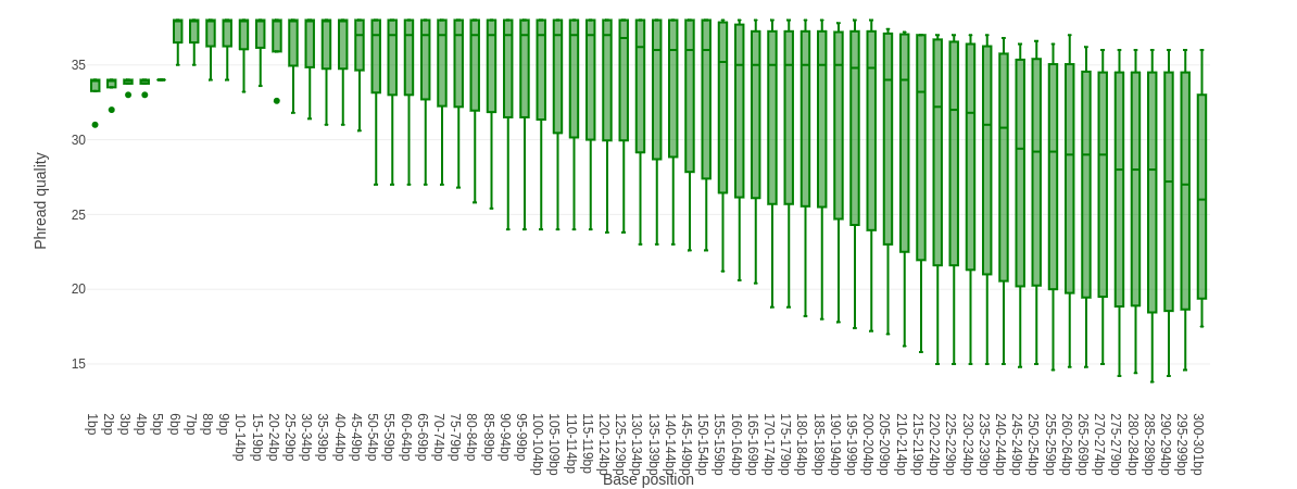
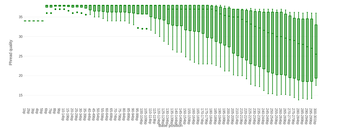
Falco combines quality statistics from all separate reads and combines them in plots. An important plot is the Per base sequence quality.
DRR187559_1
DRR187559_2
Here you have the reads sequence length on the x-axes against the quality score (Phred-score) on the y-axis. The colour of the beams indicates three quality levels:
Green = good quality,
Yellow = mediocre quality, and
Red = bad quality.
For each position, a boxplot is drawn with:
the median value, represented by the central intense coloured line
the inter-quartile range (25-75%), represented by the green, yellow or red box
the 10% and 90% values in the upper and lower whiskers
Question
How does the median quality score change along the sequence?
The median quality score (intense coloured line) decreases at the sequences end. It is common for the median quality to drop towards the end of the sequences, as the sequencers are incorporating more incorrect nucleotides at the end. For Illumina data it is normal that the first few bases are of some lower quality and how longer the reads get the worse the quality becomes. This is often due to signal decay or phasing during the sequencing run.
Quality improvement
Depending on the analysis it could be possible that a certain quality or length
is needed. In this case we are going to trim the data using fastp (Chen et al. 2018):
Trim the start and end of the reads if those fall below a quality score of 20
Different trimming tools have different algorithms for deciding when to cut but trimmomatic will cut based on the quality score of one base alone. Trimmomatic starts from each end, and as long as the base is below 20, it will be cut until it reaches one greater than 20. A sliding window trimming will be performed where if the average quality of 4 bases drops below 20, the read will be truncated there.
Filter for reads to keep only reads with at least 30 bases: Anything shorter will complicate the assembly
Hands On: Quality improvement
fastp ( Galaxy version 1.0.1+galaxy3) with the following parameters:
“Single-end or paired reads”: Paired Collection
“Select paired collection(s)”: Paired Reads
In “Filter Options”:
In “Length filtering Options”:
Length required: 30
In “Read Modification Options”:
In “Per read cuitting by quality options”:
Cut by quality in front (5’): Yes
Cut by quality in tail (3’): Yes
Cutting window size: 4
Cutting mean quality: 20
In “Output Options”:
“Output JSON report”: Yes
Edit the tags of the fastp FASTQ outputs to
Remove the #unfiltered tag
Add a new tag #filtered
fastp generates also a report, similar to Falco, useful to compare the impact of the trimming and filtering.
Question
Looking at fastp HTML report
How did the average read length change before and after filtering?
Did trimming improve the mean quality scores?
Did trimming affect the GC content?
Is this data ok to assemble? Do we need to re-sequence it?
Read lengths went down more significantly:
Before filtering: 190bp, 221bp
After filtering: 189bp, 219bp
It increased the percentage of Q20 and Q30 bases (bases with quality score above 20 and 30 respectively)
No, it did not. If it had, that would be unexpected.
This data looks OK. The number of short reads in R1 is not optimal but assembly should partially work but not the entire, closed genome.
Identification of expected species and detection of contamination
When working with bacterial isolates, it is crucial to verify whether the expected species or strains are present in the data and to identify any potential contamination. Ensuring the presence of the intended species is essential for the accuracy and reliability of the research, as deviations could lead to erroneous conclusions. Additionally, detecting contamination is vital to maintain the integrity of the samples and to avoid misleading results that could compromise subsequent analyses and applications.
Taxonomic profiling
To find out which microorganisms are present, we will compare the filtered reads of the sample to a reference database, i.e. sequences of known microorganisms stored in a database, using Kraken2 (Wood et al. 2019).
In the \(k\)-mer approach for taxonomy classification, we use a database containing DNA sequences of genomes whose taxonomy we already know. On a computer, the genome sequences are broken into short pieces of length \(k\) (called \(k\)-mers), usually 30bp.
Kraken examines the \(k\)-mers within the query sequence, searches for them in the database, looks for where these are placed within the taxonomy tree inside the database, makes the classification with the most probable position, then maps \(k\)-mers to the lowest common ancestor (LCA) of all genomes known to contain the given \(k\)-mer.
Kraken2 uses a compact hash table, a probabilistic data structure that allows for faster queries and lower memory requirements. It applies a spaced seed mask of s spaces to the minimizer and calculates a compact hash code, which is then used as a search query in its compact hash table; the lowest common ancestor (LCA) taxon associated with the compact hash code is then assigned to the k-mer.
For this tutorial, we will use the PlusPF database which contains the RefSeq Standard (archaea, bacteria, viral, plasmid, human, UniVec_Core), protozoa and fungi data.
Hands On: Assign taxonomic labels with Kraken2
Kraken2 ( Galaxy version 2.1.3+galaxy2) with the following parameters:
“Single or paired reads”: Paired
“Collection of paired reads”: fastpPaired-end output
“Minimum Base Quality”: 10
In “Create Report”:
“Print a report with aggregrate counts/clade to file”: Yes
“Select a Kraken2 database”: PlusPF-16
Kraken2 generates 2 outputs:
Classification: tabular files with one line for each sequence classified by Kraken and 5 columns:
C/U: a one letter indicating if the sequence classified or unclassified
Sequence ID as in the input file
NCBI taxonomy ID assigned to the sequence, or 0 if unclassified
Length of sequence in bp (read1|read2 for paired reads)
A space-delimited list indicating the lowest common ancestor (LCA) mapping of each k-mer in the sequence
For example, 562:13 561:4 A:31 0:1 562:3 would indicate that:
The first 13 k-mers mapped to taxonomy ID #562
The next 4 k-mers mapped to taxonomy ID #561
The next 31 k-mers contained an ambiguous nucleotide
The next k-mer was not in the database
The last 3 k-mers mapped to taxonomy ID #562
|:| indicates end of first read, start of second read for paired reads
Report: tabular files with one line per taxon and 6 columns or fields
Percentage of fragments covered by the clade rooted at this taxon
Number of fragments covered by the clade rooted at this taxon
Number of fragments assigned directly to this taxon
A rank code, indicating
(U)nclassified
(R)oot
(D)omain
(K)ingdom
(P)hylum
(C)lass
(O)rder
(F)amily
(G)enus, or
(S)pecies
Taxa that are not at any of these 10 ranks have a rank code that is formed by using the rank code of the closest ancestor rank with a number indicating the distance from that rank. E.g., G2 is a rank code indicating a taxon is between genus and species and the grandparent taxon is at the genus rank.
NCBI taxonomic ID number
Indented scientific name
 Column 1	Column 2	Column 3	Column 4	Column 5	Column 6
 0.24 	1065 	1065 	U 	0 	unclassified
 99.76 	450716 	14873 	R 	1 	root
 96.44 	435695 	2 	R1 	131567 	cellular organisms
 96.44 	435675 	3889 	D 	2 	Bacteria
 95.56 	431709 	78 	D1 	1783272 	Terrabacteria group
 95.53 	431578 	163 	P 	1239 	Firmicutes
 95.49 	431390 	4625 	C 	91061 	Bacilli
 94.38 	426383 	1436 	O 	1385 	Bacillales
 94.04 	424874 	2689 	F 	90964 	Staphylococcaceae
 93.44 	422124 	234829 	G 	1279 	Staphylococcus
Question
How many taxa have been found?
What are the percentage on unclassified?
What are the domains found?
627, as the number of lines
0.24%
Only Bacteria
Species identification
In Kraken output, there are quite a lot of identified taxa with different levels. To obtain a more accurate and detailed understanding at the species level, we will use Bracken.
Bracken refines the Kraken results by re-estimating the abundances of species in metagenomic samples, providing a more precise and reliable identification of species, which is crucial for downstream analysis and interpretation.
Bracken (Bayesian Reestimation of Abundance after Classification with Kraken) is a “simple and worthwile addition to Kraken for better abundance estimates” (Ye et al. 2019). Instead of only using proportions of classified reads, it takes a probabilistic approach to generate final abundance profiles. It works by re-distributing reads in the taxonomic tree: “Reads assigned to nodes above the species level are distributed down to the species nodes, while reads assigned at the strain level are re-distributed upward to their parent species” (Lu et al. 2017).
Hands On: Extract species with Bracken
Bracken ( Galaxy version 3.1+galaxy0) with the following parameters:
param-collection“Kraken report file”: Report output of Kraken
“Select a kmer distribution”: PlusPF-16, same as for Kraken
It is important to choose the same database that you also chose for Kraken2
“Level”: Species
“Produce Kraken-Style Bracken report”: Yes
Bracken generates 2 outputs:
Kraken style report: tabular files with one line per taxon and 6 columns or fields. Same configuration as the Report output of Kraken:
Percentage of fragments covered by the clade rooted at this taxon
Number of fragments covered by the clade rooted at this taxon
Number of fragments assigned directly to this taxon
A rank code, indicating
(U)nclassified
(R)oot
(D)omain
(K)ingdom
(P)hylum
(C)lass
(O)rder
(F)amily
(G)enus, or
(S)pecies
NCBI taxonomic ID number
Indented scientific name
 Column 1	Column 2	Column 3	Column 4	Column 5	Column 6
 100.00 	450408 	0 	R 	1 	root
 99.14 	446538 	0 	R1 	131567 	cellular organisms
 99.14 	446524 	0 	D 	2 	Bacteria
 99.14 	446524 	0 	D1 	1783272 	Terrabacteria group
 99.13 	446491 	0 	P 	1239 	Firmicutes
 99.13 	446491 	0 	C 	91061 	Bacilli
 99.06 	446152 	0 	O 	1385 	Bacillales
 99.06 	446152 	0 	F 	90964 	Staphylococcaceae
 99.04 	446101 	0 	G 	1279 	Staphylococcus
 95.62 	430661 	430661 	S 	1280 	Staphylococcus aureus
Question
How many taxa have been found?
What is the family found?
119, as the number of lines
Staphylococcaceae, with 99.06%!
Report: tabular files with one line per taxon and 7 columns or fields
Taxon name
Taxonomy ID
Level ID (S=Species, G=Genus, O=Order, F=Family, P=Phylum, K=Kingdom)
Which the species has been the most identified? And in which proportion?
What are the other species?
51 (52 lines including 1 line with header)
Staphylococcus aureus with 95.6% of the reads.
Most of the other species are from Staphylococcus genus, so same as Staphylococcus aureus. The other species in really low proportion.
As expected Staphylococcus aureus represents most of the reads in the data.
Contamination detection
To explore Kraken report and specially to detect more reliably minority organisms or contamination, we will use Recentrifuge (Martı́ Jose Manuel 2019).
Recentrifuge enhances analysis by reanalyzing metagenomic classifications with interactive charts that highlight confidence levels. It supports 48 taxonomic ranks of the NCBI Taxonomy, including strains, and generates plots for shared and exclusive taxa, facilitating robust comparative analysis.
Recentrifuge includes a novel contamination removal algorithm, useful when negative control samples are available, ensuring data integrity with control-subtracted plots. It also excels in detecting minority organisms in complex datasets, crucial for sensitive applications such as clinical and environmental studies.
Hands On: Identify contamination
Recentrifuge ( Galaxy version 1.16.1+galaxy0) with the following parameters:
param-collection“Select taxonomy file tabular formated”: Classification output of Kraken2tool
“Type of input file (Centrifuge, CLARK, Generic, Kraken, LMAT)”: Kraken
In “Database type”:
“Cached database whith taxa ID”: NCBI-2023-06-27
In “Output options”:
“Type of extra output to be generated (default on CSV)”: TSV
“Remove the log file”: Yes
In ” Fine tuning of algorithm parameters”:
“Strain level instead of species as the resolution limit for the robust contamination removal algorithm; use with caution, this is an experimental feature”: Yes
Recentrifuge generates 3 outputs:
A statistic table with general statistics about assignations
Question
How many sequences have been used?
How many sequences have been classified?
451,780
450,715
A data table with a report for each taxa
Question
How many taxa have been kept?
What is the lowest level in the data?
187 (190 lines including 3 header lines)
The lowest level is strain.
A HTML report with a Krona chart
Question
What is the percentage of classified sequences?
When clicking on Staphylococcus aureus, what can we say about the strains?
Is there any contamination?
99.8%
99% of sequences assigned to Staphylococcus aureus are not assigned to any strains, probably because they are too similar to several strains. Staphylococcus aureus subsp. aureus JKD6159 is the strain with the most classified sequences, but only 0.3% of the sequences assigned to Staphylococcus aureus.
There is no sign of a possible contamination. Most sequences are classified to taxon on the Staphylococcus aureus taxonomy. Only 3% of the sequences are not classified to Staphylococcus.
Once we have identified contamination, if any is present, the next step is to remove the contaminated sequences from the dataset to ensure the integrity of the remaining data. This can be done using bioinformatics tools designed to filter out unwanted sequences, such as BBduk (Bushnell et al. 2017).
BBduktool is a member of the BBTools package, where ‘Duk’ stands for Decontamination Using Kmers. BBduk filters or trims reads for adapters and contaminants using k-mers, effectively removing unwanted sequences and improving the quality of the dataset.
Additionally, it’s important to document and report the contamination findings to maintain transparency and guide any necessary adjustments in sample collection or processing protocols.
Conclusion
In this tutorial, we inspected the quality of the bacterial isolate sequencing data and checked the expected species and potential contamination. Prepared short reads can be used in downstream analysis, like Genome Assembly. Even after the assembly, you can identify contamination using a tool like CheckM (Parks et al. 2015). CheckMtool can be used for screening the ‘cleanness’ of bacterial assemblies.
To learn more about data quality control, you can follow this tutorial: Quality Control.
You've Finished the Tutorial
Please also consider filling out the Feedback Form as well!
Key points
Conduct quality control on every dataset before performing any other bioinformatics analysis
Review the quality metrics and, if necessary, improve the quality of your data
Check the impact of the quality control
Detect witch microorganisms are present and extract the species level
Check possible contamination in a bacterial isolate
Frequently Asked Questions
Have questions about this tutorial? Have a look at the available FAQ pages and support channels
Further information, including links to documentation and original publications, regarding the tools, analysis techniques and the interpretation of results described in this tutorial can be found here.
References
Wood, D. E., and S. L. Salzberg, 2014 Kraken: ultrafast metagenomic sequence classification using exact alignments. Genome Biology 15: R46. 10.1186/gb-2014-15-3-r46
Parks, D. H., M. Imelfort, C. T. Skennerton, P. Hugenholtz, and G. W. Tyson, 2015 CheckM: assessing the quality of microbial genomes recovered from isolates, single cells, and metagenomes. Genome Research 25: 1043–1055. 10.1101/gr.186072.114
Bushnell, B., J. Rood, and E. Singer, 2017 BBMerge - Accurate paired shotgun read merging via overlap (P. J. Biggs, Ed.). 12: e0185056. 10.1371/journal.pone.0185056
Lu, J., F. P. Breitwieser, P. Thielen, and S. L. Salzberg, 2017 Bracken: estimating species abundance in metagenomics data. PeerJ Computer Science 3: e104. 10.7717/peerj-cs.104
Chen, S., Y. Zhou, Y. Chen, and J. Gu, 2018 fastp: an ultra-fast all-in-one FASTQ preprocessor. 10.1093/bioinformatics/bty560
Hikichi, M., M. Nagao, K. Murase, C. Aikawa, T. Nozawa et al., 2019 Complete Genome Sequences of Eight Methicillin-Resistant Staphylococcus aureus Strains Isolated from Patients in Japan (I. L. G. Newton, Ed.). Microbiology Resource Announcements 8: 10.1128/mra.01212-19
Martı́ Jose Manuel, 2019 Recentrifuge: Robust comparative analysis and contamination removal for metagenomics. PLoS computational biology 15: e1006967. 10.1371/journal.pcbi.100696
Wood, D. E., J. Lu, and B. Langmead, 2019 Improved metagenomic analysis with Kraken 2. Genome biology 20: 1–13. 10.1186/s13059-019-1891-0
Ye, S. H., K. J. Siddle, D. J. Park, and P. C. Sabeti, 2019 Benchmarking Metagenomics Tools for Taxonomic Classification. Cell 178: 779–794. 10.1016/j.cell.2019.07.010
Feedback
Did you use this material as an instructor? Feel free to give us feedback on how it went.
Did you use this material as a learner or student? Click the form below to leave feedback.
Hiltemann, Saskia, Rasche, Helena et al., 2023 Galaxy Training: A Powerful Framework for Teaching! PLOS Computational Biology 10.1371/journal.pcbi.1010752
Batut et al., 2018 Community-Driven Data Analysis Training for Biology Cell Systems 10.1016/j.cels.2018.05.012
@misc{sequence-analysis-quality-contamination-control,
author = "Bérénice Batut and Clea Siguret",
	title = "Quality and contamination control in bacterial isolate using Illumina MiSeq Data (Galaxy Training Materials)",
	year = "",
	month = "",
	day = "",
	url = "\url{https://training.galaxyproject.org/training-material/topics/sequence-analysis/tutorials/quality-contamination-control/tutorial.html}",
	note = "[Online; accessed TODAY]"
}
@article{Hiltemann_2023,
	doi = {10.1371/journal.pcbi.1010752},
	url = {https://doi.org/10.1371%2Fjournal.pcbi.1010752},
	year = 2023,
	month = {jan},
	publisher = {Public Library of Science ({PLoS})},
	volume = {19},
	number = {1},
	pages = {e1010752},
	author = {Saskia Hiltemann and Helena Rasche and Simon Gladman and Hans-Rudolf Hotz and Delphine Larivi{\`{e}}re and Daniel Blankenberg and Pratik D. Jagtap and Thomas Wollmann and Anthony Bretaudeau and Nadia Gou{\'{e}} and Timothy J. Griffin and Coline Royaux and Yvan Le Bras and Subina Mehta and Anna Syme and Frederik Coppens and Bert Droesbeke and Nicola Soranzo and Wendi Bacon and Fotis Psomopoulos and Crist{\'{o}}bal Gallardo-Alba and John Davis and Melanie Christine Föll and Matthias Fahrner and Maria A. Doyle and Beatriz Serrano-Solano and Anne Claire Fouilloux and Peter van Heusden and Wolfgang Maier and Dave Clements and Florian Heyl and Björn Grüning and B{\'{e}}r{\'{e}}nice Batut and},
	editor = {Francis Ouellette},
	title = {Galaxy Training: A powerful framework for teaching!},
	journal = {PLoS Comput Biol}
}
Funding
These individuals or organisations provided funding support for the development of this resource
Questions:

 of the genomes that contain that k-mer in the database. The taxa associated with the sequence's k-mers, as well as the taxa's ancestors, form a pruned subtree of the general taxonomy tree, which is used for classification. In the classification tree, each node has a weight equal to the number of k-mers in the sequence associated with the node's taxon. Each root-to-leaf (RTL) path in the classification tree is scored by adding all weights in the path, and the maximal RTL path in the classification tree is the classification path (nodes highlighted in yellow). The leaf of this classification path (the orange, leftmost leaf in the classification tree) is the classification used for the query sequence. Source: <span class=\"citation\"><a href=\"#Wood2014\">Wood and Salzberg 2014</a></span>")