This tutorial will take you from raw FASTQ files to a cell x gene data matrix in AnnData format. What’s a data matrix, and what’s AnnData format? Well you’ll find out! Importantly, this is the first step in processing single cell data in order to start analysing it.
You are in one of the four tutorials associated with a Case Study, which replicates and expands on the analysis performed in a manuscript Bacon et al. 2018.
Figure 1: Overview of the four parts of the case study, represented by boxes connected with noodles. There is a signpost specifying that you are currently in the first part.
Currently you have a bunch of strings of ATGGGCTT etc. in your sequencing files, and what you need to know is how many cells you have and what genes appear in those cells. These steps are the most computationally heavy in the single cell world, as you’re starting with 100s of millions of reads, each with 4 lines of text. Later on in analysis, this data becomes simple gene counts such as ‘Cell A has 4 GAPDHs’, which is a lot easier to store! Because of this data overload, we have downsampled the FASTQ files to speed up the analysis a bit. Saying that, you’re still having to map loads of reads to the massive murine genome, so get yourself a cup of coffee and prepare to analyse!
Warning: For the bench scientists and biologists!
If you’re not used to computing, this tutorial will not feel intuitive. It’s lots of heavy (and necessary) computational steps with little visible reward. You will still absolutely be able to complete it, but it won’t make that much sense.
That is ok!
Conceptually, the levelFilter, plot & explore tutorial (which comes later) is when you really get to generate fun plots and interpret them scientifically. However, you can’t do that until you have pre-processed your data. Some learners like doing that tutorial first, them coming back to learn how to build their input dataset here. So:
If you’re in a Live course, follow the path of training materials
If you’re learning on your own, either get through these pre-processing steps with the belief that plots will get more fun later, or:
Try out the levelFilter, plot & explore tutorial first, then swing back and do this one.
It’s up to you!
Tools are frequently updated to new versions. Your Galaxy may have multiple versions of the same tool available. By default, you will be shown the latest version of the tool. This may NOT be the same tool used in the tutorial you are accessing. Furthermore, if you use a newer tool in one step, and try using an older tool in the next step… this may fail! To ensure you use the same tool versions of a given tutorial, use the Tutorial mode feature.
Open your Galaxy server
Click on the curriculum icon on the top menu, this will open the GTN inside Galaxy.
Navigate to your tutorial
Tool names in tutorials will be blue buttons that open the correct tool for you
Note: this does not work for all tutorials (yet)
You can click anywhere in the grey-ed out area outside of the tutorial box to return back to the Galaxy analytical interface
Warning: Not all browsers work!
We’ve had some issues with Tutorial mode on Safari for Mac users.
Try a different browser if you aren’t seeing the button.
Did you know we have a unique Single Cell Omics Lab with all our single cell tools highlighted to make it easier to use on Galaxy? We recommend this site for all your single cell analysis needs, particularly for newer users.
The Single Cell Omics Lab is a different view of the underlying Galaxy server that organises tools and resources better for single-cell users! It also provides a platform for communities to engage and connect; distribute more targeted news and events; and highlight community-specific funding sources.
When something goes wrong in Galaxy, there are a number of things you can do to find out what it was. Error messages can help you figure out whether it was a problem with one of the settings of the tool, or with the input data, or maybe there is a bug in the tool itself and the problem should be reported. Below are the steps you can follow to troubleshoot your Galaxy errors.
Expand the red history dataset by clicking on it.
Sometimes you can already see an error message here
View the error message by clicking on the bug icongalaxy-bug
Check the logs. Output (stdout) and error logs (stderr) of the tool are available:
Expand the history item
Click on the details icon
Scroll down to the Job Information section to view the 2 logs:
If you get stuck, you can first check your history against an galaxy-history-answer Answer Key history found in the header of (some) tutorials.
First, import the target history.
Open the link to the shared history
Click on the Import this history button on the top left
Enter a title for the new history
Click on Copy History
Next, compare the answer key history with your own history.
You can view multiple Galaxy histories at once. This allows to better understand your analyses and also makes it possible to drag datasets between histories. This is called “History multiview”. The multiview can be enabled either view History menu or via the Activity Bar:
Option 1: Enabling Multiview via History menu is done by first clicking on the galaxy-history-options “History options” drop-down and selecting galaxy-multihistory “Show Histories Side-by-Side option”:
Option 2: Clicking the galaxy-multihistory “History Multiview” button within the Activity Bar:
You can compare there, or if you’re really stuck, you can also click and drag a given dataset to your history to continue the tutorial from there.
There 3 ways to copy datasets between histories
From the original history
Click on the galaxy-gear icon which is on the top of the list of datasets in the history panel
Click on Copy Datasets
Select the desired files
Give a relevant name to the “New history”
Validate by ‘Copy History Items’
Click on the new history name in the green box that have just appear to switch to this history
Using the galaxy-columnsShow Histories Side-by-Side
Click on the galaxy-dropdown dropdown arrow top right of the history panel (History options)
Click on galaxy-columnsShow Histories Side-by-Side
If your target history is not present
Click on ‘Select histories’
Click on your target history
Validate by ‘Change Selected’
Drag the dataset to copy from its original history
Drop it in the target history
From the target history
Click on User in the top bar
Click on Datasets
Search for the dataset to copy
Click on its name
Click on Copy to current History
You can also use our handy troubleshooting guide.
When something goes wrong in Galaxy, there are a number of things you can do to find out what it was. Error messages can help you figure out whether it was a problem with one of the settings of the tool, or with the input data, or maybe there is a bug in the tool itself and the problem should be reported. Below are the steps you can follow to troubleshoot your Galaxy errors.
Expand the red history dataset by clicking on it.
Sometimes you can already see an error message here
View the error message by clicking on the bug icongalaxy-bug
Check the logs. Output (stdout) and error logs (stderr) of the tool are available:
Expand the history item
Click on the details icon
Scroll down to the Job Information section to view the 2 logs:
In this section, we will show you the principles of the initial phase of single-cell RNA-seq analysis: generating expression measures in a matrix. We’ll concentrate on droplet-based (rather than plate-based) methodology, since this is the process with most differences with respect to conventional approaches developed for bulk RNA-seq.
Droplet-based data consists of three components: cell barcodes, unique molecular identifiers (UMIs) and cDNA reads. To generate cell-wise quantifications we need to:
Process cell barcodes, working out which ones correspond to ‘real’ cells, which to sequencing artefacts, and possibly correct any barcodes likely to be the product of sequencing errors by comparison to more frequent sequences.
Map biological sequences to the reference genome or transcriptome.
‘De-duplicate’ using the UMIs.
This used to be a complex process involving multiple algorithms, or was performed with technology-specific methods (such as 10X’s ‘Cellranger’ tool) but is now much simpler thanks to the advent of a few new methods. When selecting methodology for your own work you should consider:
STARsolo - a droplet-based scRNA-seq-specific variant of the popular genome alignment method STAR. Produces results very close to those of Cellranger (which itself uses STAR under the hood).
Kallisto/ bustools - developed by the originators of the transcriptome quantification method, Kallisto.
Alevin - another transcriptome analysis method developed by the authors of the Salmon tool.
We’re going to use Alevin Srivastava et al. 2019 for demonstration purposes, but we do not endorse one method over another.
Get Data
We’ve provided you with some example data to play with, a small subset of the reads in a mouse dataset of fetal growth restriction ()Bacon et al. 2018). You can also find it in the study in Single Cell Expression Atlas and in Array Express), where we downloaded the original FASTQ files.zs This is a study using the Drop-seq chemistry, however this tutorial is almost identical to a 10x chemistry. We will point out the one tool parameter change you will need to run 10x samples. This data is not carefully curated, standard tutorial data - it’s real, it’s messy, it desperately needs filtering, it has background RNA running around, and most of all it will give you a chance to practice your analysis as if this data were yours.
Down-sampled reads and some associated annotation will be imported in your first step.
The datasets take a while to run in their original size, so we’ve pre-selected 400,000 lines from the original file to make it run faster. How did we do this?
How did I downsample these FASTQ files? You can check out the galaxy-history [ ] ( https://singlecell.usegalaxy.eu/u/wendi.bacon.training/h/cs1pre-processing-with-alevin—input-1 ) to find out!
warning If you are in a live course, the time to explore this downsampling history is not be factored into the schedule. Please instead check it out after your course is finished, or if you finish early!
Additionally, to map your reads, we have given you a transcriptome to align against (a FASTA) as well as the gene information for each transcript (a gtf) file.
In practice, you can download the latest, most accurate files for your species of interest from Ensembl.
Hands-on: Choose Your Own Tutorial
This is a 'Choose Your Own Tutorial' (CYOT) section (also known as 'Choose Your Own Analysis' (CYOA)), where you can select between multiple paths. Click one of the buttons below to select how you want to follow the tutorial
If you’re on the EU server, (if your usegalaxy has an EU anywhere in the URL), then the quickest way to Get the Data for this tutorial is via importing a history. Otherwise, you can import from Zenodo.
Hands On: Import History from EU server
Import the galaxy-history-inputInput history by following the link below
Click galaxy-uploadUpload at the top of the activity panel
Select galaxy-wf-editPaste/Fetch Data
Paste the link(s) into the text field
Press Start
Close the window
Rename galaxy-pencil the datasets: Change SLX-7632.TAAGGCGA.N701.s_1.r_1.fq-400k to N701-Read1 and SLX-7632.TAAGGCGA.N701.s_1.r_2.fq-400k.fastq to N701-Read2.
Question
Have a look at the files you now have in your history.
Which of the FASTQ files do you think contains the barcode sequences?
Given the chemistry this study should have, are the barcode/UMI reads the correct length?
What is the ‘N701’ referring to?
Read 1 (SLX-7632.TAAGGCGA.N701.s_1.r_1.fq-400k) contains the cell barcode and UMI because it is significantly shorter (indeed, 20 bp!) compared to the longer, r_2 transcript read. For ease, it’s better to rename these files N701-Read1 and N701-Read2.
You can see Read 1 is only 20 bp long, which for original Drop-Seq is 12 bp for cell barcode and 8 bp for UMI. This is correct! Be warned - 10x Chromium (and many technologies) change their chemistry over time, so particularly when you are accessing public data, you want to check and make sure you have your numbers correct!
‘N701’ is referring to an index read. This sample was run alongside 6 other samples, each denoted by an Illumina Nextera Index (N70X). Later, this will tell you batch information. If you look at the ‘Experimental Design’ file, you’ll see that the N701 sample was from a male wildtype neonatal thymus.
Gene-level, rather than transcript-level, quantification is standard in scRNA-seq, which means that the expression level of alternatively spliced RNA molecules are combined to create gene-level values. Droplet-based scRNA-seq techniques only sample one end each transcript, so lack the full-molecule coverage that would be required to accurately quantify different transcript isoforms.
Generate a transcript to gene map
To generate gene-level quantifications based on transcriptome quantification, Alevin and similar tools require a conversion between transcript and gene identifiers. We can derive a transcript-gene conversion from the gene annotations available in genome resources such as Ensembl. The transcripts in such a list need to match the ones we will use later to build a binary transcriptome index. If you were using spike-ins, you’d need to add these to the transcriptome and the transcript-gene mapping.
In your example data you will see the murine reference annotation as retrieved from Ensembl in GTF format. This annotation contains gene, exon, transcript and all sorts of other information on the sequences. We will use these to generate the transcript/ gene mapping by passing that information to a tool that extracts just the transcript identifiers we need.
Question
Which of the ‘attributes’ in the last column of the GTF files contains the transcript and gene identifiers?
The file is organised such that the last column (headed ‘Group’) contains a wealth of information in the format: attribute1 “information associated with attribute 1”;attribute2 “information associated with attribute 2” etc.
gene_id and transcript_id are each followed by “ensembl gene_id” and “ensembl transcript_id”
It’s now time to parse (computing term for separating out important information from a larger file) the GTF file using the rtracklayer package in R. This parsing will give us a conversion table with a list of transcript identifiers and their corresponding gene identifiers for counting. Additionally, because we will be generating our own binary index (more later!), we also need to input our FASTA so that it can be filtered to only contain transcriptome information found in the GTF.
Hands On: Generate a filtered FASTA and transcript-gene map
GTF2GeneList ( Galaxy version 1.52.0+galaxy0) with the following parameters:
param-file“Ensembl GTF file”: GTF file in the historygalaxy-history
“Feature type for which to derive annotation”: transcript (Your sequences are transcript sequencing, so this is your starting point)
“Field to place first in output table”: transcript_id (This is accessing the column you identified above!)
“Suppress header line in output?”: galaxy-toggleYes (The next tool (Alevin) does not expect a header)
“Comma-separated list of field names to extract from the GTF (default: use all fields)”: transcript_id,gene_id (This calls the first column to be the transcript_id, and the second the gene_id. Thus, your key can turn transcripts into genes)
“Append version to transcript identifiers?”: galaxy-toggleYes (The Ensembl FASTA files usually have these, and since we need the FASTA transcriptome and the GTF gene information to work together, we need to append these!)
“Flag mitochondrial features?”: galaxy-toggleNo
“Provide a cDNA file for extracting annotations and/ or possible filtering?”: galaxy-toggleYes
param-file“FASTA-format cDNA/transcript file”: Mus_musculus.GRCm38cdna.all.fa (you may have renamed your differently in your galaxy-history history)
“Annotation field to match with sequences”: transcript_id
“Filter the cDNA file to match the annotations?”: galaxy-toggleYes
Rename galaxy-pencil the annotation table to Map
Rename galaxy-pencil the filtered FASTA file to Filtered_FASTA
Generate a transcriptome index & quantify!
Alevin collapses the steps involved in dealing with dscRNA-seq into a single process. Such tools need to compare the sequences in your sample to a reference containing all the likely transcript sequences (a ‘transcriptome’). This will contain the biological transcript sequences known for a given species, and perhaps also technical sequences such as ‘spike ins’ if you have those.
To be able to search a transcriptome quickly, Alevin needs to convert the text (FASTA) format sequences into something it can search quickly, called an ‘index’. The index is in a binary rather than human-readable format, but allows fast lookup by Alevin. Because the types of biological and technical sequences we need to include in the index can vary between experiments, and because we often want to use the most up-to-date reference sequences from Ensembl or NCBI, we can end up re-making the indices quite often. Making these indices is time-consuming! Have a look at the uncompressed FASTA to see what it starts with.
We now have:
Barcode/ UMI reads
cDNA reads
transcript/ gene mapping
filtered FASTA
We can now run Alevin! However, Alevin will inherently do some of its own filtering and thresholding. We will actually use a better tool later (emptyDrops) that needs to work on raw outputs. Therefore, we are going to select options to limit Alevin from filtering the outputs.
Hands On: Running Alevin
Alevin ( Galaxy version 1.10.1+galaxy2)
“Select a reference transcriptome from your history or use a built-in index?”: Use one from the history
You are going to generate the binary index using your filtered FASTA!
In “Salmon index”:
param-file“Transcripts FASTA file”: Filtered_FASTA
“Single or paired-end reads?”: Paired-end
param-file“Mate pair 1”: N701-Read1
param-file“Mate pair 2”: N701-Read2
“Specify the strandedness of the reads”: Infer automatically (A)
“Type of single-cell protocol”: DropSeq Single Cell protocol
param-file“Transcript to gene map file”: Map
In “Extra output files”:
param-checkSalmon Quant log file
param-checkFeatures used by the CB classification and their counts at each cell level (--dumpFeatures)
In “Advanced options”:
” Dump cell v transcripts count matrix in MTX format”: galaxy-toggleYes
“Fraction of cellular barcodes to keep”: 1.0 (this prevents Alevin from adding extra thresholds!)
“Minimum frequency for a barcode to be considered”: 3 (This is normally set at about 10, but as we’ve downsampled these datasets, setting it to 10 would pretty much delete them!)
The main parameter that needs changing for a 10X Chromium sample is the ‘Protocol’ parameter of Alevin. Just select the correct 10x Chemistry there instead.
The Salmon documentation on ‘Fragment Library Types’ and running the Alevin command is here: salmon.readthedocs.io/en/latest/library_type.html and salmon.readthedocs.io/en/latest/alevin.html. These links will help here, although keep in mind the image there is drawn with the RNA 5’ on top, whereas in this scRNA-seq protocol, the polyA is captured by its 3’ tail and thus effectively the bottom or reverse strand…)
Comment: Alevin file names
You will notice that the names of the output files of Alevin are written in a certain convention, mentioning which tool was used and on which files, for example: “Alevin on data X, data Y, and others: whitelist”. Remember that you can always rename the files if you wish! For simplicity, when we refer to those files in the tutorial, we skip the information about tool and only use the second part of the name - in this case it would be simply “whitelist”.
This tool will take a while to run. Alevin produces many file outputs, not all of which we’ll use. You can refer to the Alevin documentation if you’re curious what they all are, but we’re most interested in is:
the matrix itself (per-cell gene-count matrix (MTX) - the count by gene and cell)
the row (cell/ barcode) identifiers (row index (CB-ids)) and
the column (gene) labels (column headers (gene-ids)).
Question
After you’ve run Alevin, galaxy-eye look through all the different output files. Can you find:
The Mapping Rate?
How many cells are present in the matrix output?
Inspect galaxy-eye the file param-fileSalmon log file. You can see the mapping rate is a paltry 48.3268% (This may vary slightly with tool versions). This is not a great mapping rate. Why might this be? For early Drop-Seq samples and single-cell data in general, you might expect a slightly poorer mapping rate. 10x samples are much better these days! This is real data, not test data, after all!
Peek at the file param-filerow index (CB-ids) in your galaxy-history, and you will find it has 22,952 lines. The rows refer to the cells in the cell x gene matrix. According to this (rough) estimate, your sample has 22,952 cells in it! This entirely inaccurate, because it’s currently counting background noise as cells. So we need to do some Quality Control (QC)!
congratulations Congratulations - you’ve made an expression matrix! We could almost stop here. But it’s sensible to do some basic QC, and one of the things we can do is look at a barcode rank plot.
Generating QC Plots
The question we’re looking to answer here, is: “do we mostly have a single cell per droplet”? That’s what experimenters are normally aiming for, but it’s not entirely straightforward to get exactly one cell per droplet. Sometimes almost no cells make it into droplets, other times we have too many cells in each droplet. At a minimum, we should easily be able to distinguish droplets with cells from those without.
Hands On: Generate a raw barcode QC plot
Droplet barcode rank plot ( Galaxy version 1.6.1+galaxy2) with the following parameters:
“Input MTX-format matrix?”: galaxy-toggleNo
param-file“A two-column tab-delimited file, with barcodes in the first column and frequencies in the second”: Output of Alevin raw CB classification frequencies
“Label to place in plot title”: Barcode rank plot (raw barcode frequencies)
Rename galaxy-pencil the image output Barcode Plot - raw barcode frequencies
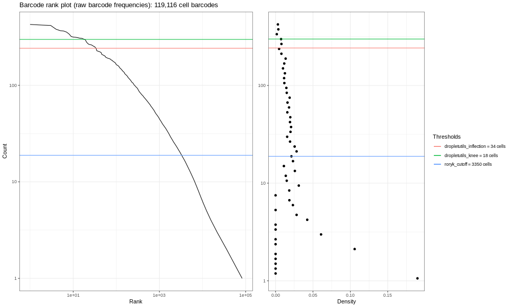
Interpreting the QC plots
This is our own formulation of the barcode plot based on a discussion we had with community members. The left hand plots with the smooth lines are the main plots, showing the UMI counts for individual cell barcodes ranked from high to low. The right hand plots are density plots from the first one, and the thresholds are generated either using dropletUtils or by the method described in the discussion mentioned above.
Now, the image generated here (400k) isn’t the most informative - but you are dealing with a fraction of the reads! If you run the total sample (so identical steps above, but with significantly more time!) you’d get the image below.
We expect a sharp drop-off between cell-containing droplets and ones that are empty or contain only cell debris. Then, various proposed thresholds (shown in the different coloured horizontal lines) are calculated by Alevin, to give options of where to put a cut-off line that says “Any barcodes with fewer reads per cell than this cut-off line are discarded, because these are likely background and uninformative.” Ideally, this cut-off is clearly at the point where the curve bends, known as the knee of the curve.
Now, this data is not an ideal dataset, so for perspective, in an ideal world with a very clean 10x run, data will look a bit more like the following taken from the lung atlas (see the study in Single Cell Expression Atlas and the project submission).
You can see the clearer ‘knee’ bend in this significantly larger and cleaner sample, showing the cut-off between empty droplets and cell-containing droplets.
While we could use any of these calculated thresholds to select cells, there are some more sophisticated methods also available. We will try one called “emptyDrops”.
emptyDrops
In experiments with relatively simple characteristics, the ‘knee detection’ method works relatively well. But some populations (such as our sample!) present difficulties. For instance, sub-populations of small cells may not be distinguished from empty droplets based purely on counts by barcode. Some libraries produce multiple ‘knees’ for multiple sub-populations. The emptyDrops method has become a popular way of dealing with this. emptyDrops still retains barcodes with high counts, but also adds in barcodes that can be statistically distinguished from the ambient profiles, even if total counts are similar.
Reformatting for emptyDrops
Alevin outputs MTX format. However, emptyDrops runs on SingleCellExperiment (SCE) format. To get there, we will perform the following steps:
Swap Cells & Genes orientation
Add in gene metadata (gene symbols, mitochondrial information)
Convert to a SingleCellExperiment object
Transform matrix
First, we need to ‘transform’ the matrix such that cells are in columns and genes are in rows.
Hands On: Transform matrix
salmonKallistoMtxTo10x ( Galaxy version 0.0.1+galaxy6) with the following parameters:
param-file“.mtx-format matrix”: per-cell gene-count matrix (MTX) (output of Alevintool)
param-file“Tab-delimited genes file”: column headers (gene-ids) (output of Alevintool)
param-file“Tab-delimited barcodes file”: row index (CB-ids) (output of Alevintool)
Rename galaxy-pencil ‘salmonKallistoMtxTo10x….:genes’ to Gene_table
Rename galaxy-pencil ‘salmonKallistoMtxTo10x….:barcodes’ to Barcode_table
Rename galaxy-pencil ‘salmonKallistoMtxTo10x….:matrix’ to Matrix_table
The output is a matrix in the correct orientation for the rest of our tools. However, our matrix is looking a bit sparse - for instance, click on Gene_table. I don’t know about you, but I’d struggle to have a good biological discussion using only Ensembl gene_ids! What I’d really like is the more understandable ‘GAPDH’ or other gene acronym, as well as information on mitochondrial genes so that I can assess if my cells were stressed out or not. In order to prepare our data for emptyDrops, we’re going to combine this information into an object, and it’s easiest to add in that information now.
Add in Gene metadata
Question
Where can we find information about genes?
Our old friend the GTF file!
Question
Which of the ‘attributes’ in the last column of that file contains the gene acronym?
gene_name
We’re now going to re-run galaxy-refresh the tool that extracts information from our GTF file, but extract gene information instead of transcript information.
Hands On: Generate gene information
GTF2GeneList ( Galaxy version 1.52.0+galaxy0) with the following parameters:
“Feature type for which to derive annotation”: gene
“Field to place first in output table”: gene_id
“Suppress header line in output?”: galaxy-toggleYes
“Comma-separated list of field names to extract from the GTF (default: use all fields)”: gene_id,gene_name,mito
“Append version to transcript identifiers?”: galaxy-toggleYes
“Flag mitochondrial features?”: galaxy-toggleYes - note, this will auto-fill a bunch of acronyms for searching in the GTF for mitochondrial associated genes. This is good!
“Filter the cDNA file to match the annotations?”: galaxy-toggleNo - we don’t need to, we’re done with the FASTA!
Convert the param-file annotation table (TSV) output to tabular
Click on the galaxy-pencilpencil icon for the dataset to edit its attributes
In the central panel, click galaxy-chart-select-dataDatatypes tab on the top
In the galaxy-chart-select-dataAssign Datatype, select tabular from “New Type” dropdown
Tip: you can start typing the datatype into the field to filter the dropdown menu
Click the Save button
Rename galaxy-pencil the tabular annotation table to Gene_Information
Inspect galaxy-eye the param-fileGene_Information object in the history. You have made a new key for gene_id, with gene name and a column of mitochondrial information (false = not mitochondrial, true = mitochondrial). We need to add this information into the param-file salmonKallistoMtxTo10x output Gene_table. But we need to keep Gene_table in the same order, since it is referenced in the Matrix_table by row.
Hands On: Combine MTX Gene Table with Gene Information
Join two Datasets with the following parameters:
“Join”: Gene_table
“Using column”: Column: 1
“with”: Gene_Information
“and column”: Column: 1
“Keep lines of first input that do not join with second input”: Yes
“Keep lines of first input that are incomplete”: Yes
“Fill empty columns”: No
“Keep the header lines”: No
If you inspect galaxy-eye the object, you’ll see we have joined these tables and now have quite a few gene_id repeats. Let’s take those out, while keeping the order of the original ‘Gene Table’.
Cut columns from a table with the following parameters:
“Cut columns”: c1,c4,c5
“Delimited by”: Tab
“From”: output of Join two Datasetstool
Rename output Annotated_Gene_Table
Inspect galaxy-eye your Annotated_Gene_Table. That’s more like it! You now have gene_id, gene_name, and mito information (just without a header to label them). Now let’s get back to your journey to emptyDrops and sophisticated thresholding of empty droplets!
Convert to SCE format
The tool emptyDrops Lun et al. 2019 works with a specific form of R object called a “SingleCellExperiment”. We need to convert our transformed MTX files into that form, using the DropletUtils Read10x tool:
Hands On: Converting to SingleCellExperiment format
DropletUtils Read10x ( Galaxy version 1.0.4+galaxy0) with the following parameters:
param-file“Expression matrix in sparse matrix format (.mtx)”: Matrix_table
param-file“Gene Table”: Annotated_Gene_Table
param-file“Barcode/cell table”: Barcode_table
“Should metadata file be added?”: galaxy-toggleNo
Rename galaxy-pencil output: SCE_Object
Fantastic! Now that our matrix is combined into an object, specifically the SingleCellExperiment format, we can now run emptyDrops! Let’s get rid of those background droplets containing no cells!
Run emptyDrops
Hands On: Emptydrops
DropletUtils emptyDrops ( Galaxy version 1.0.4+galaxy0) with the following parameters:
“Should barcodes estimated to have no cells be removed from the output object?”: galaxy-toggleYes
Rename galaxy-pencilserialised SingleCellExperiment output as Emptied_Object
Question
How many cell barcodes remain after the emptyDrops treatment? Why might that be?
If you peek at the Emptied_Object in your galaxy-history history, the text in that window says 38 barcodes or something similar to that - there is an element of random in the algorithm, so yours might differ slightly. Why is this so low?? And why might the number be different?
Consider…is this a complete set of data?
Remember this is a subsampled dataset. If you look carefully at the parameters of emptyDrops, you’ll see it set a minimum threshold at 100 UMI. If you look at the barcode plots above for the 400k read sample, you’ll see this is far too stringent for this subsampled data! To satisfy your curiosity, this minimum threshold would yield around 4332 barcodes for the total sample. Again, the number may vary slightly as the output depends on a large number of random iterations.
We will nevertheless proceed with your majestic annotated expression matrix of ~38 cells, ready to go for further processing and analysis!
Hands-on: Choose Your Own Tutorial
This is a 'Choose Your Own Tutorial' (CYOT) section (also known as 'Choose Your Own Analysis' (CYOA)), where you can select between multiple paths. Click one of the buttons below to select how you want to follow the tutorial
Which toolsuite do you intend to use to analyse your data? Both Scanpy and Seurat are supported in Galaxy. We probably have slightly more tools for Scanpy in Galaxy at the time of writing, so we will default to that, but pick what works for you!
The tool suite called Scanpy (Wolf et al. 2018) uses a format called AnnData, which is a variant of a file format called hdf5. You will now convert your SCE object to an AnnData one!
Convert to AnnData object
Hands On: Converting to AnnData format
SCEasy Converter ( Galaxy version 0.0.7+galaxy2) with the following parameters:
“Convert From / To”: SingleCellExperiment to AnnData
param-file“Input object in sce,rds,rdata.sce format”: Emptied_Object
If the dataset does not show up in the corresponding input field or displays as ‘unavailable’, don’t worry - try dragging the dataset from the history panel and dropping it into the input field. If this still doesn’t work, then you can change the datatype to rdata.sce.
Click on the galaxy-pencilpencil icon for the dataset to edit its attributes
In the central panel, click galaxy-chart-select-dataDatatypes tab on the top
In the galaxy-chart-select-dataAssign Datatype, select your desired datatype from “New Type” dropdown
Tip: you can start typing the datatype into the field to filter the dropdown menu
Click the Save button
Last but not least, after all these data conversions, your AnnData object is missing some labelling. If you peek at our latest output param-file in your galaxy-history history, and check the vars categories, you will find one category labelled NA. What is this? To find out, you can use a handy tool.
Hands On: Inspecting AnnData Objects
Inspect AnnData ( Galaxy version 0.10.9+galaxy1) with the following parameters:
param-file“Annotated data matrix”: output_anndata (output of SCEasy Convertertool)
“What to inspect?”: Key-indexed annotation of variables/features (var)
If you galaxy-eye examine the output param-file, you will find that this NA. column is a bunch of True/False outputs.
Question
What are this “True/False” referring to? (Hint: Consider what gene information you have added!)
The second time you ran the GTF2GeneList, you extracted gene_id,gene_name,mito information and then added that information to your datasets. The mito flagging outputs a True if the gene has any mitochondrial information in its GTF listing, or False if it does not. Therefore, this NA. should be labelled mito!
Flag mitochondrial genes
Hands On: Label Mito Metadata
Manipulate AnnData ( Galaxy version 0.10.9+galaxy1) with the following parameters:
param-file“Annotated data matrix”: output_anndata (output of SCEasy Convertertool)
“Function to manipulate the object”: Rename fileds in AnnData variables
“Name of the variables field that you want to change”: NA.
“New name of the filed in the variables”: mito
Rename galaxy-pencil output N701-400k-AnnData
Your object is ready to for the scanpy pipeline!
Conclusion
congratulations Congrats! You have finished the tutorial!
We have:
Examined raw read data, annotations and necessary input files for quantification.
Run Alevin and applied emptyDrops instead of Alevin’s inbuilt thresholds.
Deployed barcode rank plots as a way of quickly assessing the signal present in droplet datasets.
Converted these datasets to enable downstream analysis.
You might find the galaxy-history-answerAnswer Key Histories helpful to check or compare with:
It may be that you want to combine this object with others like it, for instance, maybe you ran 5 samples, and you are starting with 10 FASTQ files… To do this, you can run that same Workflow on all your files! In fact, that’s what we do to set up the datasets for the next tutorial. You can explore applying this tutorial to all seven samples in this dataset, either in the downsampled or whole state.
warning Remember that if you are in a course, time for exploring these histories will not be factored into the schedule. Explore these outside of course time!
We also post new tutorials / workflows there from time to time, as well as any other news.
point-right If you’d like to contribute ideas, requests or feedback as part of the wider community building single-cell and spatial resources within Galaxy, you can also join our Single cell & sPatial Omics Community of Practice.
Further information, including links to documentation and original publications, regarding the tools, analysis techniques and the interpretation of results described in this tutorial can be found here.
References
Bacon, W. A., R. S. Hamilton, Z. Yu, J. Kieckbusch, D. Hawkes et al., 2018 Single-Cell Analysis Identifies Thymic Maturation Delay in Growth-Restricted Neonatal Mice. Frontiers in Immunology 9: 10.3389/fimmu.2018.02523
Wolf, F. A., P. Angerer, and F. J. Theis, 2018 SCANPY: large-scale single-cell gene expression data analysis. Genome Biology 19: 10.1186/s13059-017-1382-0
Lun, A., S. Riesenfeld, T. Andrews, T. Dao, T. Gomes et al., 2019 EmptyDrops: Distinguishing cells from empty droplets in droplet-based single-cell RNA sequencing data. Genome Biology 20: 63. 10.1186/s13059-019-1662-y
Srivastava, A., L. Malik, T. Smith, I. Sudbery, and R. Patro, 2019 Alevin efficiently estimates accurate gene abundances from dscRNA-seq data. Genome Biology 20: 10.1186/s13059-019-1670-y
Feedback
Did you use this material as an instructor? Feel free to give us feedback on how it went.
Did you use this material as a learner or student? Click the form below to leave feedback.
Hiltemann, Saskia, Rasche, Helena et al., 2023 Galaxy Training: A Powerful Framework for Teaching! PLOS Computational Biology 10.1371/journal.pcbi.1010752
Batut et al., 2018 Community-Driven Data Analysis Training for Biology Cell Systems 10.1016/j.cels.2018.05.012
@misc{single-cell-scrna-case_alevin,
author = "Wendi Bacon and Jonathan Manning",
	title = "Generating a single cell matrix using Alevin (Galaxy Training Materials)",
	year = "",
	month = "",
	day = "",
	url = "\url{https://training.galaxyproject.org/training-material/topics/single-cell/tutorials/scrna-case_alevin/tutorial.html}",
	note = "[Online; accessed TODAY]"
}
@article{Hiltemann_2023,
	doi = {10.1371/journal.pcbi.1010752},
	url = {https://doi.org/10.1371%2Fjournal.pcbi.1010752},
	year = 2023,
	month = {jan},
	publisher = {Public Library of Science ({PLoS})},
	volume = {19},
	number = {1},
	pages = {e1010752},
	author = {Saskia Hiltemann and Helena Rasche and Simon Gladman and Hans-Rudolf Hotz and Delphine Larivi{\`{e}}re and Daniel Blankenberg and Pratik D. Jagtap and Thomas Wollmann and Anthony Bretaudeau and Nadia Gou{\'{e}} and Timothy J. Griffin and Coline Royaux and Yvan Le Bras and Subina Mehta and Anna Syme and Frederik Coppens and Bert Droesbeke and Nicola Soranzo and Wendi Bacon and Fotis Psomopoulos and Crist{\'{o}}bal Gallardo-Alba and John Davis and Melanie Christine Föll and Matthias Fahrner and Maria A. Doyle and Beatriz Serrano-Solano and Anne Claire Fouilloux and Peter van Heusden and Wolfgang Maier and Dave Clements and Florian Heyl and Björn Grüning and B{\'{e}}r{\'{e}}nice Batut and},
	editor = {Francis Ouellette},
	title = {Galaxy Training: A powerful framework for teaching!},
	journal = {PLoS Comput Biol}
}
Congratulations on successfully completing this tutorial!
Do you want to extend your knowledge?
Follow one of our recommended follow-up trainings:
5 stars:
Liked: I would happy in next year continue with this course
September 2024
4 stars:
Liked: Explains why we perform each step
Disliked: My brain! The course is fine as it is
March 2022
5 stars:
Liked: Everything because all were new for me
Disliked: To be given the ability to conduct all parts of the tutorial, because some tools (in my condition) were not worked and I had to create a new account on another server in order to fulfill the tutorial.
January 2022
2 stars:
Disliked: The examples are still very buggy. Many of them do not work with the instructions as supplied. For example, the SalmonKallistoMtxTo10x instructions fails, most likely because the program is looking for a gz file when the tutorial example makes an unzipped file. The Droplet barcode rank plot exercise also crashes.
November 2021
5 stars:
Liked: The instructions are clear, I really enjoyed it thank you!
Disliked: Notes for the versions of the tools so you can select them and go a little bit faster with the course.
July 2021
3 stars:
Disliked: Speak a bit slower and explain each file before moving on. Relate the theoretical apresentation with this part.
Questions:
Open image in new tab


 Open image in new tab
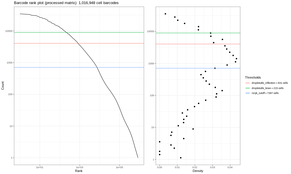 Open image in new tab
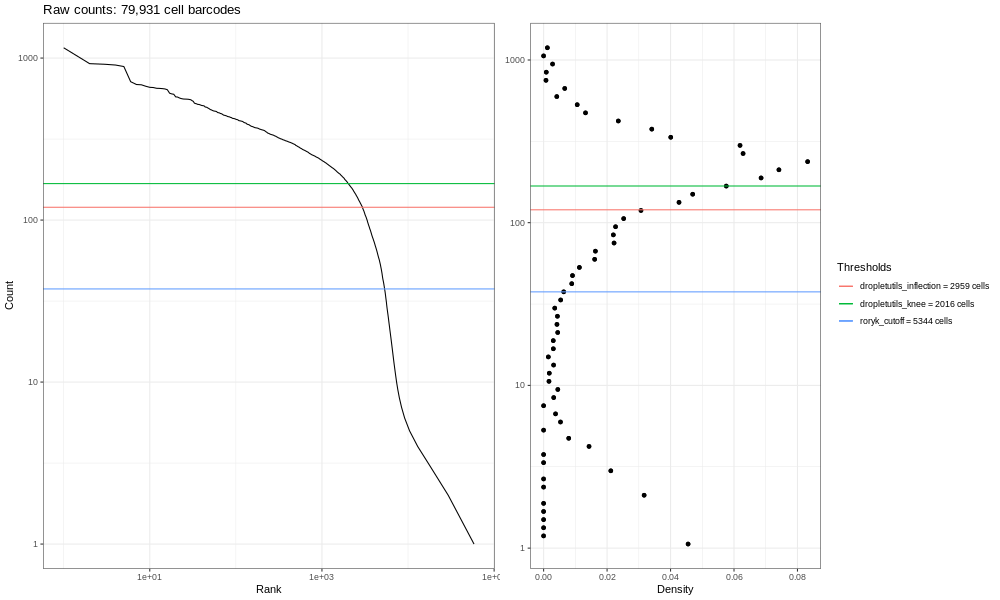 Open image in new tab