Hi-C analysis of Drosophila melanogaster cells using HiCExplorer
| Author(s) |
|
| Editor(s) |
|
| Reviewers |
|
OverviewQuestions:
Objectives:
Why is a Hi-C analysis useful?
What is ‘chromosome conformation capture’?
What are main steps in order to generate and plot a Hi-C contact matrix?
Requirements:
- Introduction to Galaxy Analyses
- slides Slides: Quality Control
- tutorial Hands-on: Quality Control
- slides Slides: Mapping
- tutorial Hands-on: Mapping
Time estimation: 2 hoursSupporting Materials:Published: Feb 23, 2018Last modification: Mar 16, 2026License: Tutorial Content is licensed under Creative Commons Attribution 4.0 International License. The GTN Framework is licensed under MITpurl PURL: https://gxy.io/GTN:T00141rating Rating: 3.8 (0 recent ratings, 9 all time)version Revision: 31
In this HiCExplorer tutorial we will generate and plot a Hi-C contact matrix. For this the following steps are necessary to be performed:
- Map the Hi-C reads to the reference genome
- Creation of a Hi-C matrix
- Plotting the Hi-C matrix
- Correction of Hi-C matrix
- TAD Calling
- A/B compartments computation
- pyGenomeTracks visualization
- Loop detection
After a corrected Hi-C matrix is created other tools can be used to visualise it, call TADS or compare it with other matrices.
AgendaIn this tutorial, we will deal with:
Data upload
Hands On: Data upload
Create a new history
To create a new history simply click the new-history icon at the top of the history panel:
Import from Zenodo.
https://zenodo.org/records/16416373/files/HiC_S2_1p_10min_lowU_R1.fastq.gz
https://zenodo.org/records/16416373/files/HiC_S2_1p_10min_lowU_R2.fastq.gz
- Copy the link location
Click galaxy-upload Upload at the top of the activity panel
- Select galaxy-wf-edit Paste/Fetch Data
Paste the link(s) into the text field
Press Start
- Close the window
Rename galaxy-pencil the data set to something meaningful
- e.g.
HiC_S2_1p_10min_lowU_R1andHiC_S2_1p_10min_lowU_R2.- By default, when data is imported via its link, Galaxy names it with its URL.
- Click on the galaxy-pencil pencil icon for the dataset to edit its attributes
- In the central panel, change the Name field
- Click the Save button
Comment: Get data from public sourcesHiCExplorer needs as input the forward and reverse strand of a pair end read which are mapped independently. A usual start point for a typical analysis is the given GSE number of a publication, e.g. GSE63525 for Rao 2014. To get the actual data, go to NCBI and search for the GSE number. In the section ‘Samples’ the GSM numbers of all samples are given. Select the correct one for you, and go to the European Nucleotide Archive and enter the GSM number. Select a matching result e.g. SRX764936 and download the data given in the row ‘FASTQ files (FTP)’ the forward and reverse strand. It is important to have the forward and reverse strand individual as a FASTQ file and to map it individually, HiCExplorer can not work with interleaved files.

Reads mapping
Mates have to be mapped individually to avoid mapper specific heuristics designed for standard paired-end libraries.
We have used the HiCExplorer successfully with bwa, bowtie2 and hisat2. In this tutorial we will be using Bowtie2 tool. It is important to remember to:
- use local mapping, in contrast to end-to-end. A fraction of Hi-C reads are chimeric and will not map end-to-end thus, local mapping is important to increase the number of mapped reads
- tune the aligner parameters to penalize deletions and insertions. This is important to avoid aligned reads with gaps if they happen to be chimeric.
- If bowtie2 or hisat2 are used,
--reorderoption and as a file formatbam_nativeneeds to be used. Regularbamfiles are sorted by Galaxy and can not be used as an input for HiCExplorer.
Hands On: Mapping reads
Bowtie2( Galaxy version 2.5.3+galaxy1): RunBowtie2on both strandsHiC_S2_1p_10min_lowU_R1andHiC_S2_1p_10min_lowU_R2with:
- “Is this single or paired library”:
Single-end- Set multiple data sets
- “FASTQ file”:
HiC_S2_1p_10min_lowU_R1andHiC_S2_1p_10min_lowU_R2- “Will you select a reference genome from your history or use a built-in index?”:
Use a built-in index- “Select a reference genome”:
dm3- “Do you want to tweak SAM/BAM Options?”:
Yes
- “Reorder output to reflect order of the input file”:
Yes- Rename galaxy-pencil the output of the tool according to the corresponding files:
R1.bamandR2.bam
Creating a Hi-C matrix
Once the reads have been mapped the Hi-C matrix can be built.
For this step we will use hicBuildMatrix tool, which builds the matrix of read counts over the bins in the genome, considering the sites around the given restriction site.
For versions 3.6 and later, hicBuildMatrix requires an input BED file that specifies the locations of all restriction cuts. We must first identify restriction enzyme sites use the tool hicFindRestSite, which requires a fasta file containing the genome of organism we are studying. We will import the dm3_genome.fasta genome file from Zenodo.
Hands On: Import from Zenodo
- Import the reference genome
https://zenodo.org/records/16416373/files/dm3_genome.fasta
- Copy the link location
Click galaxy-upload Upload at the top of the activity panel
- Select galaxy-wf-edit Paste/Fetch Data
Paste the link(s) into the text field
Press Start
- Close the window
Hands On: Find Restriction Sites and Build Matrix
hicFindRestSite( Galaxy version 3.7.6+galaxy1):
- “Fasta file for the organism genome.”:
dm3_genome.fasta“Restriction enzyme sequence”:
GATCCommentOur data uses the DpnII restriction enzyme, which has the Restriction enzyme sequence:
GATC. The Restriction enzyme sequence will be specific to the restriction enzyme that your data uses (e.g. for HindIII this will beAAGCTT).Rename galaxy-pencil the output to
Restriction Sites.hicBuildMatrix( Galaxy version 3.7.6+galaxy1): RunhicBuildMatrixon theR1.bamandR2.bammapping output.
- “1: Sam/Bam files to process (forward/reverse)”:
R1.bam- “2: Sam/Bam files to process (forward/reverse)”:
R2.bam- “BED file with all restriction cut places”:
Restriction sites- “Sequence of the restriction site”:
GATC- “Dangling sequence”:
GATC“Bin size in bp”:
10000CommenthicBuildMatrix creates two files, a bam file containing only the valid Hi-C read pairs and a matrix containing the Hi-C contacts at the given resolution. The bam file is useful to check the quality of the Hi-C library on the genome browser. A good Hi-C library should contain piles of reads near the restriction fragment sites. In the QC folder a html file is saved with plots containing useful information for the quality control of the Hi-C sample like the number of valid pairs, duplicated pairs, self-ligations etc. Usually, only 25%-40% of the reads are valid and used to build the Hi-C matrix mostly because of the reads that are on repetitive regions that need to be discarded.
CommentNormally 25% of the total reads are selected. The output matrices have counts for the genomic regions. The extension of output matrix files is .h5. A quality report is created in e.g.
hicMatrix/R1_10kb_QC, have a look at the report hicQC.html.- Rename galaxy-pencil the output to
10kb contact matrix.
CommentIf you do not have access to the genome for your organism (e.g. if you plan to use your Hi-C data to assist with genome assembly) then you can instead select
hicBuildMatrixversion 3.4.3.0.Hands On: Build Hi-C Matrix
hicBuildMatrix( Galaxy version 3.4.3.0): RunhicBuildMatrixon theR1.bamandR2.bammapping output.
- “1: Sam/Bam files to process”:
R1.bam- “2: Sam/Bam files to process”:
R2.bam- “Choose to use a restriction cut file or a bin size”:
Bin size- “Bin size in bp”:
10000- “Sequence of the restriction site”:
GATC
Plotting the Hi-C matrix
A 10 kb bin matrix is too large to plot, it’s better to reduce the resolution. We usually run out of memory for a 1 kb or a 10 kb bin matrix and the time to plot it is very long (minutes instead of seconds). In order to reduce the resolution we use the tool hicMergeMatrixBins.
hicMergeMatrixBins merges the bins into larger bins of given number (specified by –numBins). We will merge 100 bins in the original (uncorrected) matrix and then correct it. The new bin size is going to be 10.000 bp * 100 = 1.000.000 bp = 1 Mb
Hands On: Merge Matrix Bins
hicMergeMatrixBins( Galaxy version 3.7.6+galaxy1):
- “Matrix to compute on”:
10kb contact matrix- “Number of bins to merge”:
100Rename galaxy-pencil the output to
1MB contact matrix.hicPlotMatrix( Galaxy version 3.4.3.0):
- “Matrix to compute on”:
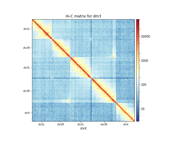
1MB contact matrix- “Plot title”:
Hi-C matrix for dm3- “Remove masked bins from the matrix”:
Yes- “Plot the log1p of the matrix values”:
Yes- “Chromosomes to include (and order to plot in)”:
chr2L- ”+ Insert Chromosomes to include (and order to plot in):”:
chr2R- ”+ Insert Chromosomes to include (and order to plot in):”:
chr3L- ”+ Insert Chromosomes to include (and order to plot in):”:
chr3R- ”+ Insert Chromosomes to include (and order to plot in):”:
chrXBecause of the large differences in counts found in the matrix, it is better to plot the counts using the
–log1poption.
The resulting plot of the 1 Mb contact matrix should look like:
Correcting the Hi-C matrix
hicCorrectMatrix corrects the matrix counts in an iterative manner. For correcting the matrix, it’s important to remove the unassembled scaffolds (e.g. NT_) and keep only chromosomes, as scaffolds create problems with matrix correction. Therefore we use the chromosome names (chr2R, chr2L, chr3R, chr3L, chrX) here.
Matrix correction works in two steps: first a histogram containing the sum of contact per bin (row sum) is produced. This plot needs to be inspected to decide the best threshold for removing bins with lower number of reads. The second steps removes the low scoring bins and does the correction.
Hands On: Matrix diagnostic
hicCorrectMatrix( Galaxy version 3.7.6+galaxy1):
- “Matrix to compute on”:
10kb contact matrix- “Range restriction (in bp)”:
Diagnostic plot- “Chromosomes to include (and order to plot in)”:
chr2L- ”+ Insert Chromosomes to include (and order to plot in):”:
chr2R- ”+ Insert Chromosomes to include (and order to plot in):”:
chr3L- ”+ Insert Chromosomes to include (and order to plot in):”:
chr3R- ”+ Insert Chromosomes to include (and order to plot in):”:
chrX
The output of the program prints a threshold suggestion that is usually accurate but is better to revise the histogram plot. The threshold is visualised in the plot as a blue vertical line.
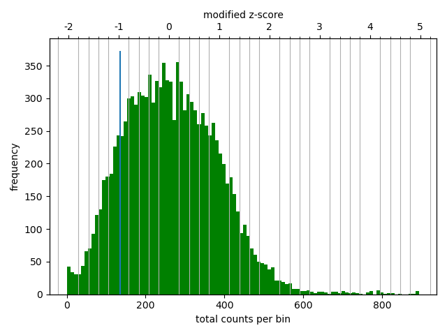
In our case the distribution describes the counts per bin of a genomic distance. To remove all bins with a z-score threshold less / more than X means to remove all bins which have less / more counts than X of mean of their specific distribution in units of the standard deviation. Looking at the distribution, we can select the value of -1.6 (lower end) and 1.8 (upper end) to remove. This is given by the –filterThreshold option in hicCorrectMatrix set to ‘correct matrix’ mode.
Hands On: Matrix correction
hicCorrectMatrix( Galaxy version 3.7.6+galaxy1):
- “Matrix to compute on”:
10kb contact matrix- “Range restriction (in bp)”:
Correct matrix- “Normalize each chromosome separately”:
Yes- “Remove bins of low coverage”:
-1.6- “Remove bins of large coverage”:
1.8- “Chromosomes to include (and order to plot in)”:
chr2L- ”+ Insert Chromosomes to include (and order to plot in):”:
chr2R- ”+ Insert Chromosomes to include (and order to plot in):”:
chr3L- ”+ Insert Chromosomes to include (and order to plot in):”:
chr3R- ”+ Insert Chromosomes to include (and order to plot in):”:
chrX- Rename galaxy-pencil the corrected matrix to
10kb corrected contact matrix.
It can happen that the correction stops with:
ERROR:iterative correction:*Error* matrix correction produced extremely large values.
This is often caused by bins of low counts. Use a more stringent filtering of bins.
This can be solved by a more stringent z-score values for the filter threshold or by a look at the plotted matrix. For example, chromosomes with 0 reads in its bins can be excluded from the correction by not defining it for the set of chromosomes that should be corrected (parameter ‘Include chromosomes’).
Plotting the corrected Hi-C matrix
We can now plot chromosome 2L with the corrected matrix.
Hands On: Plotting the corrected Hi-C matrix
hicPlotMatrix( Galaxy version 3.4.3.0):
- “Matrix to compute on”:
10kb corrected contact matrix- “Plot title”:
Hi-C matrix for dm3- “Plot per chromosome”:
No- “Plot only this region”:
chr2L- “Plot the log1p of the matrix values”:
True
Load new data
The steps so far would have led to long run times if real data would have been used. We therefore prepared a new matrix for you, corrected contact matrix dm3 large. Please import it into your history from Zenodo.
Hands On: Import from Zenodo
- Import the following file into your history:
https://zenodo.org/records/16416373/files/corrected_contact_matrix_dm3_large.h5
TAD calling
“The partitioning of chromosomes into topologically associating domains (TADs) is an emerging concept that is reshaping our understanding of gene regulation in the context of physical organization of the genome” (Ramírez et al. 2017).
TAD calling works in two steps: First HiCExplorer computes a TAD-separation score based on a z-score matrix for all bins. Then those bins having a local minimum of the TAD-separation score are evaluated with respect to the surrounding bins to assign a p-value. Then a cutoff is applied to select the bins more likely to be TAD boundaries.
hicFindTADs tries to identify sensible parameters but those can be change to identify more stringent set of boundaries.
Hands On: Finding TADs
hicFindTADs( Galaxy version 3.7.6+galaxy1):
- “Matrix to compute on”:
corrected_contact_matrix_dm3_large.h5- “Minimum window length (in bp) to be considered to the left and to the right of each Hi-C bin.”:
30000- “Maximum window length (in bp) to be considered to the left and to the right of each Hi-C bin.”:
100000- “Step size when moving from minDepth to maxDepth”:
10000- “Multiple Testing Corrections”:
False discovery rate- “q-value”:
0.05- “Minimum threshold of the difference between the TAD-separation score of a putative boundary and the mean of the TAD-sep. score of surrounding bins.”:
0.001- Rename galaxy-pencil the TAD boundary positions to
Boundary positions.- Rename galaxy-pencil the multi-scale TAD scores matrix to
Matrix with multi-scale TAD scores.- Rename galaxy-pencil the TAD domains to
TAD domains.- Rename galaxy-pencil the boundary information to
Boundary information plus score.- Rename galaxy-pencil the TAD information in bm file to
TAD information in bm file.
As an output we get the boundaries, domains and scores separated files. We will use in the plot later only the TAD-score file.
A/B compartments computation
Hands On: Computing A / B compartments
hicPCA( Galaxy version 3.7.6+galaxy1):
- “Matrix to compute on”:
corrected_contact_matrix_dm3_large.h5- “Output file format”:
bigwig- “Return internally used Pearson matrix”:
Yes- Rename galaxy-pencil the Pearson matrix to
Pearson matrix.
Hands On: Plotting the pearson matrix and PCA track
hicPlotMatrix( Galaxy version 3.4.3.0):
- “Matrix to compute on”:
Pearson matrix- “Plot title”:
Pearson matrix and PC1- “Chromosomes to include”:
chr2L- “Color map to use for the heatmap”:
gist_heat- “Plot the log1p of the matrix values (log(Hi-C contacts+1))”:
Yes- “Datatype of eigenvector file”:
bigwig- “Eigenvector file”:
pca1hicPlotMatrix( Galaxy version 3.4.3.0):
- “Matrix to compute on”:
Pearson matrix- “Plot title”:
Pearson matrix and PC2- “Chromosomes to include”:
chr2L- “Color map to use for the heatmap”:
gist_heat- “Plot the log1p of the matrix values (log(Hi-C contacts+1))”:
Yes- “Datatype of eigenvector file”:
bigwig- “Eigenvector file”:
pca2
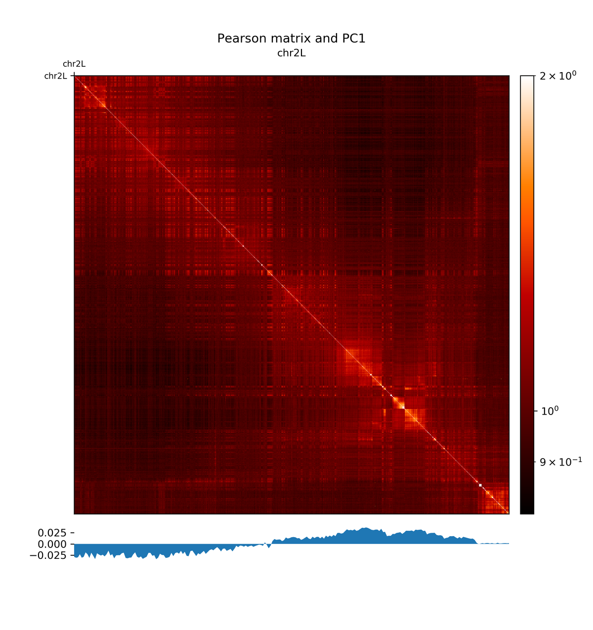
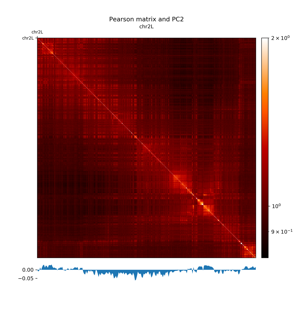
The first principal component correlates with the chromosome arms, while the second component correlates with A/B compartments.
Integrating Hi-C and other data
We can plot the TADs for a given chromosomal region. For this we will use pyGenomeTracks. For the next step we need additional data tracks. Please import dm3_genes.bed, H3K27me3.bw, H3K36me3.bw and H4K16ac.bw to your history from Zenodo.
Hands On: Import from Zenodo
- Import the following files into Galaxy:
https://zenodo.org/records/16416373/files/dm3_genes.bed
https://zenodo.org/records/16416373/files/H3K27me3.bw
https://zenodo.org/records/16416373/files/H3K36me3.bw
https://zenodo.org/records/16416373/files/H4K16ac.bw
Hands On: Update `dm3_genes.bed` databaseIf the database for
dm3_genes.bedis not “dm3” (i.e.database "?"or a different database is listed), then the database must be updated to “dm3”.
- Click the desired dataset’s name to expand it.
Click on the “?” next to database indicator:
- In the central panel, change the Database/Build field
- Select your desired database key from the dropdown list
- Click the Save button

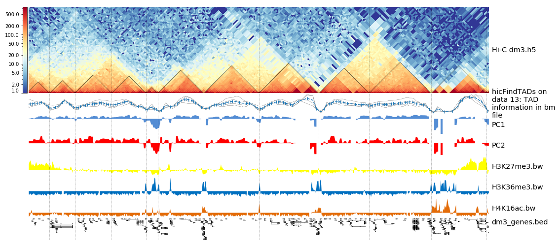
Hands On: Plotting TADs
pyGenomeTracks( Galaxy version 3.8+galaxy2):
- “Region of the genome to plot”:
chr2L:14500000-16500000- “Choose style of the track”:
TAD visualization (triangle)
- “Plot title”:
HiC dm3 chr2L:14500000-16500000- “Matricies to plot”:
corrected_contact_matrix_dm3_large.h5- “Depth”:
750000- “Height”:
4- “Boundaries file”:
TAD domains- “+Insert Include tracks in your plot”
- “Choose style of the track”:
Bedgraph matrix track/TAD score- “Plot title”:
TAD separation score- “Track file(s) bedgraph format”:
TAD information in bm file- “Height”:
4- “type of plotting”:
lines: each column in the bedgraph will be a line and a mean line will be added- “+Insert Include tracks in your plot”
- “Choose style of the track”:
Bigwig track- “Plot title”:
PC1- “Track file bigwig format”:
pca1- “Height”:
1.5- “Color of track” to a color of your choice
- “+Insert Include tracks in your plot”
- “Choose style of the track”:
Bigwig track- “Plot title”:
PC2- “Track file bigwig format”:
pca2- “Height”:
1.5- “Color of track” to a color of your choice
- “+Insert Include tracks in your plot”
- “Choose style of the track”:
Bigwig track- “Plot title”:
H3K36me3- “Track file(s) bigwig format”:
H3K36me3.bw- “Height”:
1.5- “Color of track” to a color of your choice
- “+Insert Include tracks in your plot”
- “Choose style of the track”:
Bigwig track- “Plot title”:
H3K27me3- “Track file(s) bigwig format”:
H3K27me3.bw- “Height”:
1.5- “Color of track” to a color of your choice
- “+Insert Include tracks in your plot”
- “Choose style of the track”:
Bigwig track- “Plot title”:
H4K16ac- “Track file(s) bigwig format”:
H4K16ac.bw- “Height”:
1.5- “Color of track” to a color of your choice
- “+Insert Include tracks in your plot”
- “Choose style of the track”:
Gene track / Bed track- “Plot title”:
dm3 genes- “Track file(s) bed or gtf format”:
dm3_genes.bed- “Height”:
3- “Configure other bed parameters”: - “Maximum number of gene rows”:
15- “Color of track” to a color of your choice
- “+Insert Include tracks in your plot”
- “Choose style of the track”:
Vlines track- “Track file bed format”:
TAD domains
The resulting image should look like this one:
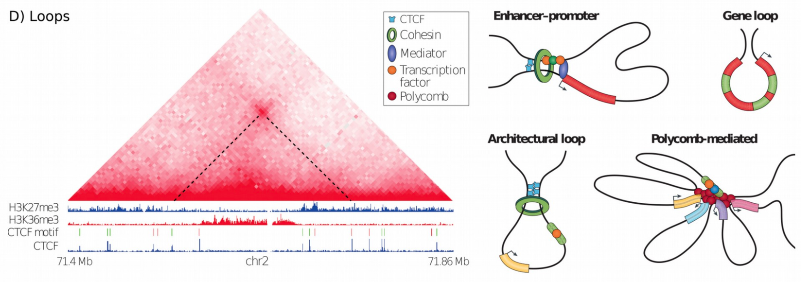
Loop detection
In Hi-C data, the term loop refers to a 3D structure which represents enhancer-promoter, gene, architectural or polycomb-mediated interactions. These interactions have the characteristics to be enriched in a single region compared to the local background. These loops are also called long-range interactions with an expected maximum distance of 2 MB (see Rao et al. 2014).
To compute loops, we will use a published Hi-C sequencing dataset from the human cell line GM12878, mapped to hg19 and of 25 kb resolution (Wolff and Heidel 2025). The original Hi-C data is from Rao et al. 2014 (GSE63525). We can import this dataset from Zenodo.
We use a new file because to detect loop structures the read coverage is required to be in the millions per chromosome; this was not the case for the previous used drosophila dataset.
Hands On: Import via URL
- Import the following file to Galaxy
https://zenodo.org/records/16416373/files/GM12878_25kb_cooler_coarsen.cool
Hands On: Matrix information
hicInfo( Galaxy version 3.7.6+galaxy1):
- “Select”
Multiple datasets- “Matrix to compute on”:
corrected_contact_matrix_dm3_large.h5andGM12878_25kb_cooler_coarsen.cool
We can view the result of hicInfo and see that the new imported file has 900 million non-zero elements, while the drosophila Hi-C interaction matrix has around 12 million non-zero elements.
We next run hicDetectLoops to find loops. In this tutorial we will only look for loops in chromosome 1 to reduce the required computational resources and computing time.
Hands On: Computing loops
hicDetectLoops( Galaxy version 3.7.6+galaxy1):
- “Matrix to compute on”:
GM12878_25kb_cooler_coarsen.cool- “Peak width”:
6- “Window size”:
10- “P-value preselection”:
0.02- “P-value”:
0.02- “Chromosomes to include”:
1
The detection of the loops is based on a pre-selection of interactions, a p-value given a continuous negative binomial distribution over all interactions of a relative distance is computed. All interactions are filtered with a threshold (p-value preselection) to retrieve loop candidates. In a second step, the selected peak candidate is compared against its background using a Wilcoxon rank-sum test.
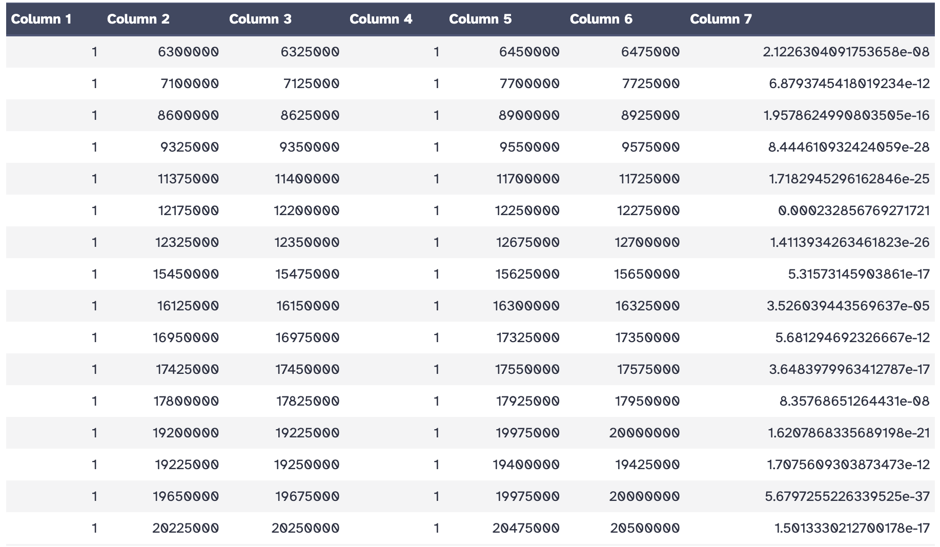
As an output we get a loop file containing the positions of both anchor points of the loop and the p-value of the used statistical test.
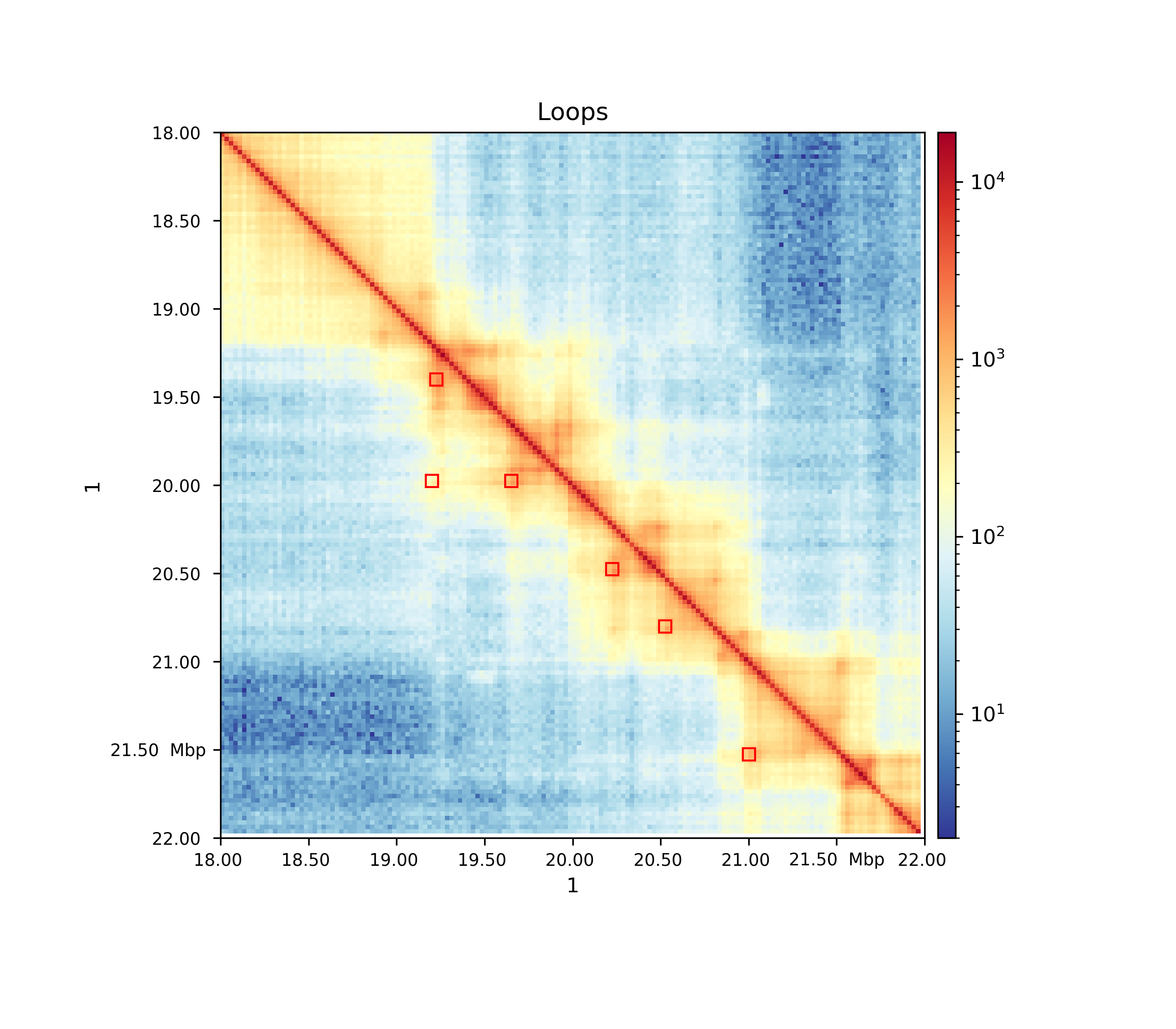
Hands On: Plotting detected loops
hicPlotMatrix( Galaxy version 3.4.3.0):
- “Matrix to compute on”:
GM12878_25kb_cooler_coarsen.cool- “Plot title”:
Loops- “Plot only this region”:
1:18000000-22000000- “Plot the log1p of the matrix values”:
Yes- “Plot Loops”:
Yes
- “Add detected loops”:
Computed loops- “DPI for image”:
300
Conclusion
In this tutorial we used HiCExplorer to analyze drosophila melanogaster cells. We mapped chimeric reads and created a contact matrix, to reduce noise this contact matrix was normalized. We showed how to visualise a contact matrix and how we can investigate topological associating domains and relate them to additional data like gene tracks. Moreover, we used a human Hi-C interaction matrix to compute loop structures.
To improve your learned skills, there is an additional hicexplorer tutorial based on mouse stem cells.
You've Finished the Tutorial
Key points
Hi-C helps to investigate the 3D structure of the genome and to uncover folding principles of chromatin.
In order to build a Hi-C contact matrix the reads have to be mapped to the reference genome.
Based on a contact matrix open and closed chromatin (A/B compartments) and topological associating domains (TADs) can be computed.
Frequently Asked Questions
Have questions about this tutorial? Have a look at the available FAQ pages and support channelsReferences
- Rao, S. S. P., M. H. Huntley, N. C. Durand, E. K. Stamenova, I. D. Bochkov et al., 2014 A 3D Map of the Human Genome at Kilobase Resolution Reveals Principles of Chromatin Looping. Cell 159: 1665–1680. 10.1016/j.cell.2014.11.021
- Ramírez, F., V. Bhardwaj, J. Villaveces, L. Arrigoni, B. A. Grüning et al., 2017 High-resolution TADs reveal DNA sequences underlying genome organization in flies. 10.1101/115063
- Wolff, J., and F. Heidel, 2025 A novel metric for hyperparameter optimization in Hi-C matrix prediction using linear regression . 10.5281/zenodo.15341976
Feedback
Did you use this material as an instructor? Feel free to give us feedback on how it went.
Did you use this material as a learner or student? Click the form below to leave feedback.

Citing this Tutorial
- Joachim Wolff, Fidel Ramirez, Vivek Bhardwaj, Ekaterina Polkh, Hi-C analysis of Drosophila melanogaster cells using HiCExplorer (Galaxy Training Materials). https://training.galaxyproject.org/training-material/topics/epigenetics/tutorials/hicexplorer/tutorial.html Online; accessed TODAY
- Hiltemann, Saskia, Rasche, Helena et al., 2023 Galaxy Training: A Powerful Framework for Teaching! PLOS Computational Biology 10.1371/journal.pcbi.1010752
- Batut et al., 2018 Community-Driven Data Analysis Training for Biology Cell Systems 10.1016/j.cels.2018.05.012
@misc{epigenetics-hicexplorer,
author = "Joachim Wolff and Fidel Ramirez and Vivek Bhardwaj and Ekaterina Polkh",
	title = "Hi-C analysis of Drosophila melanogaster cells using HiCExplorer (Galaxy Training Materials)",
	year = "",
	month = "",
	day = "",
	url = "\url{https://training.galaxyproject.org/training-material/topics/epigenetics/tutorials/hicexplorer/tutorial.html}",
	note = "[Online; accessed TODAY]"
}
@article{Hiltemann_2023,
	doi = {10.1371/journal.pcbi.1010752},
	url = {https://doi.org/10.1371%2Fjournal.pcbi.1010752},
	year = 2023,
	month = {jan},
	publisher = {Public Library of Science ({PLoS})},
	volume = {19},
	number = {1},
	pages = {e1010752},
	author = {Saskia Hiltemann and Helena Rasche and Simon Gladman and Hans-Rudolf Hotz and Delphine Larivi{\`{e}}re and Daniel Blankenberg and Pratik D. Jagtap and Thomas Wollmann and Anthony Bretaudeau and Nadia Gou{\'{e}} and Timothy J. Griffin and Coline Royaux and Yvan Le Bras and Subina Mehta and Anna Syme and Frederik Coppens and Bert Droesbeke and Nicola Soranzo and Wendi Bacon and Fotis Psomopoulos and Crist{\'{o}}bal Gallardo-Alba and John Davis and Melanie Christine Föll and Matthias Fahrner and Maria A. Doyle and Beatriz Serrano-Solano and Anne Claire Fouilloux and Peter van Heusden and Wolfgang Maier and Dave Clements and Florian Heyl and Björn Grüning and B{\'{e}}r{\'{e}}nice Batut and},
	editor = {Francis Ouellette},
	title = {Galaxy Training: A powerful framework for teaching!},
	journal = {PLoS Comput Biol}
}
Funding
These individuals or organisations provided funding support for the development of this resource


You can use Ephemeris's
shed-tools installcommand to install the tools used in this tutorial.shed-tools install [-g GALAXY] [-a API_KEY] -t <(curl https://training.galaxyproject.org/training-material/api/topics/epigenetics/tutorials/hicexplorer/tutorial.json | jq .admin_install_yaml -r)Alternatively you can copy and paste the following YAML
---
install_tool_dependencies: true
install_repository_dependencies: true
install_resolver_dependencies: true
tools:
- name: hicexplorer_hicbuildmatrix
  owner: bgruening
  revisions: 921a2da49a0c
  tool_panel_section_label: HiCExplorer
  tool_shed_url: https://toolshed.g2.bx.psu.edu/
- name: hicexplorer_hicbuildmatrix
  owner: bgruening
  revisions: d9967770de96
  tool_panel_section_label: HiCExplorer
  tool_shed_url: https://toolshed.g2.bx.psu.edu/
- name: hicexplorer_hiccorrectmatrix
  owner: bgruening
  revisions: c5ce0cbf73dc
  tool_panel_section_label: HiCExplorer
  tool_shed_url: https://toolshed.g2.bx.psu.edu/
- name: hicexplorer_hicdetectloops
  owner: bgruening
  revisions: 18bf75bf5d67
  tool_panel_section_label: HiCExplorer
  tool_shed_url: https://toolshed.g2.bx.psu.edu/
- name: hicexplorer_hicfindrestrictionsites
  owner: bgruening
  revisions: 430acc59e883
  tool_panel_section_label: HiCExplorer
  tool_shed_url: https://toolshed.g2.bx.psu.edu/
- name: hicexplorer_hicfindtads
  owner: bgruening
  revisions: 7b9fa42ca59c
  tool_panel_section_label: HiCExplorer
  tool_shed_url: https://toolshed.g2.bx.psu.edu/
- name: hicexplorer_hicinfo
  owner: bgruening
  revisions: 58293f858e2d
  tool_panel_section_label: HiCExplorer
  tool_shed_url: https://toolshed.g2.bx.psu.edu/
- name: hicexplorer_hicmergematrixbins
  owner: bgruening
  revisions: 7011782fdbaf
  tool_panel_section_label: HiCExplorer
  tool_shed_url: https://toolshed.g2.bx.psu.edu/
- name: hicexplorer_hicpca
  owner: bgruening
  revisions: 41dbf4d162a2
  tool_panel_section_label: HiCExplorer
  tool_shed_url: https://toolshed.g2.bx.psu.edu/
- name: hicexplorer_hicpca
  owner: bgruening
  revisions: b03f8b95b08c
  tool_panel_section_label: HiCExplorer
  tool_shed_url: https://toolshed.g2.bx.psu.edu/
- name: hicexplorer_hicplotmatrix
  owner: bgruening
  revisions: 5308ca68ef3d
  tool_panel_section_label: HiCExplorer
  tool_shed_url: https://toolshed.g2.bx.psu.edu/
- name: hicexplorer_hicplotmatrix
  owner: bgruening
  revisions: eb3a1b9a1c3c
  tool_panel_section_label: HiCExplorer
  tool_shed_url: https://toolshed.g2.bx.psu.edu/
- name: bowtie2
  owner: devteam
  revisions: d5ceb9f3c25b
  tool_panel_section_label: Mapping
  tool_shed_url: https://toolshed.g2.bx.psu.edu/
- name: pygenometracks
  owner: iuc
  revisions: 36b848d5f3ec
  tool_panel_section_label: Graph/Display Data
  tool_shed_url: https://toolshed.g2.bx.psu.edu/